
What is Image Augmentation?
Image augmentation is an engineered solution to create a new set of images by applying standard image processing methods to existing images.
This solution is mostly useful for neural networks or CNN when the training dataset size is small. Although, Image augmentation is also used with a large dataset as a regularization technique to build a generalized or robust model.
Deep learning algorithms are not powerful just because of their ability to mimic the human brain. They are also powerful because of their ability to thrive with more data. In fact, they require a significant amount of data to deliver considerable performance.
High performance with a small dataset is unlikely. Here, an image data augmentation technique comes in handy when we have small image data to train an algorithm.
Image augmentation techniques create different image variations from the existing set of images using the below methods:
- Image flipping
- Rotation
- Zoom
- Height and width shifting
- Perspective and tilt
- Lighting transformations
- Crop
- Noise addition
- Cutout or erasing
Content outline
Why does image augmentation work?
Image augmentation as a regularization technique
Flipping
Rotation
Zoom
Height and width shift
Tilt and perspective (shear)
Lighting transforms
Custom augmentation with preprocessing_function
Cropping
Random noise
Cutout/errasing
Training with image augmentation
Image augmentation with Keras experimental layers
Advanced custom layer for image augmentation
Before we go into much detail about how to implement the above-mentioned techniques, let’s first understand why image augmentation works.
Why does image augmentation work?
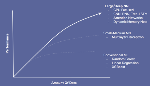
As discussed earlier, deep neural networks work best with a large amount of data. The amount of data accelerates the performance as shown below image. This image is sourced from a very informative blog on Deep Misconceptions About Deep Learning by Jesse Moore.
Here, with image augmentation, we can create numerous image variations by combining multiple of the above-mentioned transformations.
You may create 20, 25, 30, or more image variations from each image if needed. Thus, it fulfills the requirement for a fair amount of data, as you can scale your dataset 30 or more times (in a sense) using augmentation techniques.
Image data augmentation as a regularization technique
Apart from dataset scaling, image augmentation can be considered a regularization method.
A trained algorithm is required to perform well on unseen real-world data. The images attained in a real-time environment could be crazy compared to images in the training set.
These real-world images have different lighting conditions, frame position, size of an object of interest, perspective, and more.
To make algorithm learning robust, we can use these augmentations while training.
This way, the final model will be able to generalize more. I prefer to use augmentations most of the time even if the dataset is massive.
What Image Augmentation techniques are we talking about in this blog?
Here, when we talk about data augmentation, we won’t create new images and save them to storage which could also be achieved using the OpenCV library.
The OpenCV-like library will help to increase the number of images in storage but similar model performance can be obtained with in-memory image augmentation techniques.
No doubt, physical image augmentation (augmented image generation and stored on a disk) provides much more flexibility for image processing and manipulation but virtual or in-memory image augmentation is just enough for training a model.
In-memory image augmentation takes images from storage and modifies the image in real-time before feeding to neural networks while keeping the original image as it is.
In this blog, we will discuss in-memory augmentation techniques which are widely used and supported by frameworks like, Keras, tensorflow, fastai, and PyTorch.
There will be a section where we will discuss how to implement a custom augmentation based on your needs.
Here, we will list various augmentation techniques, a brief introduction, why they are used, and a code.
The code is based on the Keras library’s ImageDataGenerator class. After covering all these techniques, we will also cover the code for TensorFlow’s preprocess experimental layers for image augmentation and fastai’s image data augmentation capability.
Image Augmentation techniques
To understand how these techniques “augment” images, we will keep this article mostly visual and use many images and code. The images used here are borrowed from Pexels - free stock photos and videos portal.
Image flipping
Image flipping is the most basic type of augmentation technique. As the name suggests, it flips the image to generate an image variation.
Flipping works in two ways:
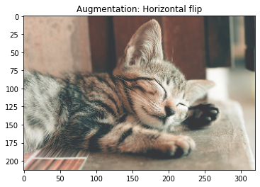
Horizontal flipping: Flips an image horizontally. Either left to right or right to left.
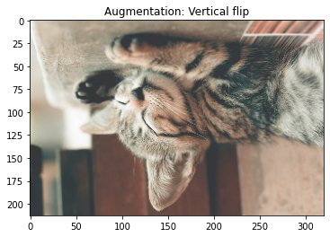
Vertical flipping: Flips an image vertically. Either up to down or down to up.
Let’s assume that we are working on a cat detection project. The data we have has few images with the right side pose of a cat. We don’t have any images with left-side orientation.
While our model is in production, there is a high probability that it might get images where a cat is in left side orientation.
Flipping images horizontally can simulate such cases. The vertical flipping can help us to train an algorithm for cases where the object of interest (i.g. a cat) could be upside down in real-world images.
Keras code for Image flip augmentation.
#importing libraries
from tensorflow.keras.preprocessing.image import ImageDataGenerator
from matplotlib import pyplot
import numpy as np
import tensorflow as tf
# downloading and saving the image
import requests
DownURL = "https://images.pexels.com/photos/1056251/pexels-photo-1056251.jpeg?crop=entropy&cs=srgb&dl=pexels-ihsan-aditya-1056251.jpg&fit=crop&fm=jpg&h=426&w=640"
img_data = requests.get(DownURL).content
with open('/tmp/impath/cat/cat-small.jpg', 'wb') as handler:
handler.write(img_data)
# setting up data pipeline to read image from disk
image_augmentor = ImageDataGenerator()
data = image_augmentor.flow_from_directory(
"/tmp/impath",
target_size=(213, 320),
batch_size=1,
)
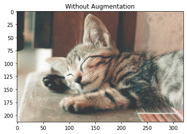
# plotting an original image
pyplot.imshow(data.next()[0][0].astype('int'))
pyplot.title("Without Augmentation")
Output:
Flow_flow_directory is a method to ImageDataGenerator class that builds a dataset from a given folder path. Learn more about the imageflow_from_directory method here.
# set up horizontal flip
image_augmentor = ImageDataGenerator(horizontal_flip=True)
data = image_augmentor.flow_from_directory(
    "/tmp/impath",
    target_size=(213, 320),
    batch_size=1,
)
pyplot.imshow(data.next()[0][0].astype('int'))
pyplot.title("Augmentation: Horizontal flip")
Output:
image_augmentor = ImageDataGenerator(vertical_flip=True)
data = image_augmentor.flow_from_directory(
    "/tmp/impath",
    target_size=(213, 320),
    batch_size=1,
)
pyplot.imshow(data.next()[0][0].astype('int'))
pyplot.title("Augmentation: Vertical flip")
Output:
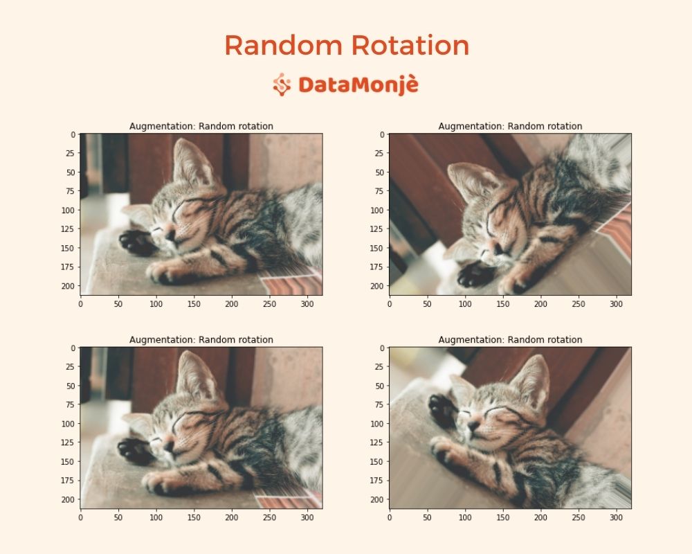
Random Image Rotation
The image rotation technique rotates an image clockwise to certain degrees.
We can configure code for random rotation from given ranges. For example, if we specify a random rotation range to 45. The images would be rotated randomly between -45 degrees to 45 degrees clockwise.
We can also configure code to rotate an image to a certain angle with a custom function e.g 5 degrees, in contrast to random rotation.
Here, if we rotate an image to 180 degrees, it will be equivalent to a vertical flip. Same way, if we rotate an image to 360 degrees, it will work as a horizontal flip.
When deployed for inference on real-world data, a trained model could get input images that are slightly angled compared to images in train data. Random rotation while training could make the model robust against such inference use cases.
# random rotation
image_augmentor = ImageDataGenerator(rotation_range=45)
data = image_augmentor.flow_from_directory(
    "/tmp/impath",
    target_size=(213, 320),
    batch_size=1,
)
pyplot.imshow(data.next()[0][0].astype('int'))
pyplot.title("Augmentation: Random rotation")
Output:
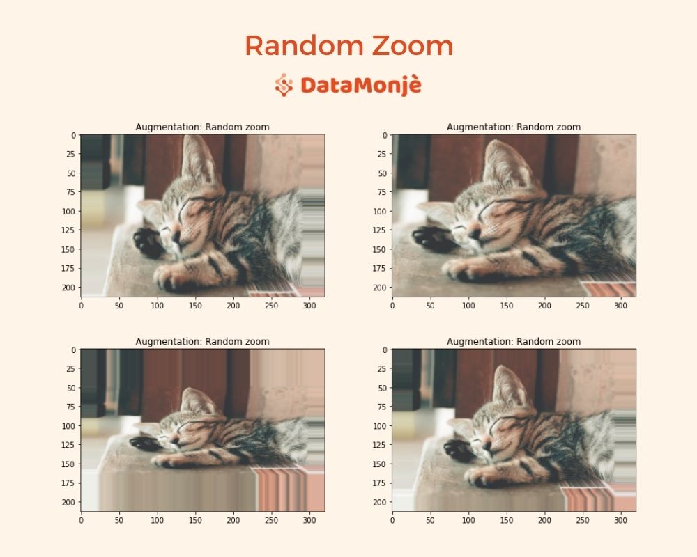
Random Image Zoom
This technique randomly zooms an image given a zooming range. Here, we can use the zoom in and zoom out both.
We can configure zooming by specifying the percentage. A percentage value less than 100% will zoom in the image and above 100% will zoom out the image.
For example, if a specified range is [0.80, 1.25], the image will be zoomed randomly from 80% to 125%.
The image input for inference might have a different scale e.g. a cat is near or far from the camera, thus the size of the cat will be large or small respectively. Image zooming will augment such scenarios.
# random zoom
# zooms an image to between 80% to 125%
image_augmentor = ImageDataGenerator(zoom_range=[0.8, 1.25])
data = image_augmentor.flow_from_directory(
    "/tmp/impath",
    target_size=(213, 320),
    batch_size=1,
)
pyplot.imshow(data.next()[0][0].astype('int'))
pyplot.title("Augmentation: Random zoom")
Output:
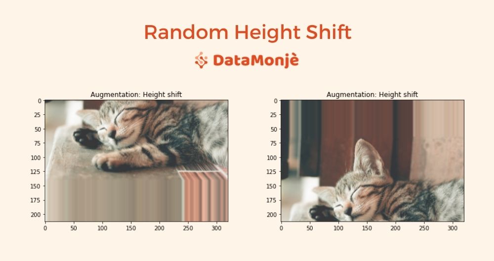
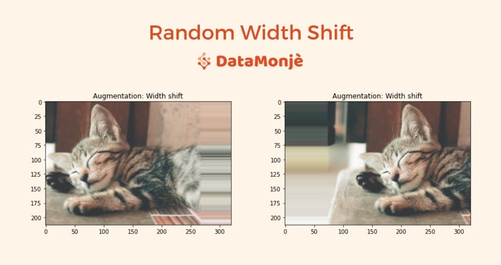
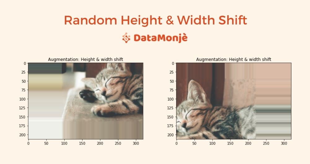
Random Height and Width Shifting
Height shifting shifts an image to up or down and width shifting shifts an image to right or left randomly.
For inference, an object of interest wouldn't always be in the center of the image. To prepare a model for such situations, with shift images in all for direction.
Keras ImageDataGenerator class allows the specification of maximum height and width shifting range. If we set height_shift_range to 200, then the image would shift randomly between 200px up to 200px down.
We can also set it to a floating number instead of an integer. A floating number of 0.20 means an image would shift a maximum of 20%.
Random Height Shift
image_augmentor = ImageDataGenerator(height_shift_range=0.30)
data = image_augmentor.flow_from_directory(
    "/tmp/impath",
    target_size=(213, 320),
    batch_size=1,
)
pyplot.imshow(data.next()[0][0].astype('int'))
pyplot.title("Augmentation: Height shift")
Output:
Random Width Shift
image_augmentor = ImageDataGenerator(width_shift_range=0.30)
data = image_augmentor.flow_from_directory(
    "/tmp/impath",
    target_size=(213, 320),
    batch_size=1,
)
pyplot.imshow(data.next()[0][0].astype('int'))
pyplot.title("Augmentation: Width shift")
Output:
Random Height & Width Shift
image_augmentor = ImageDataGenerator(width_shift_range=0.30, height_shift_range=0.30)
data = image_augmentor.flow_from_directory(
    "/tmp/impath",
    target_size=(213, 320),
    batch_size=1,
)
pyplot.imshow(data.next()[0][0].astype('int'))
pyplot.title("Augmentation: Height & width shift")
Output:
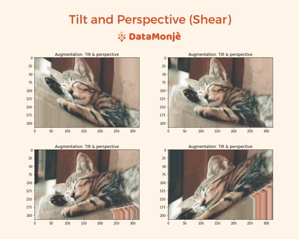
Tilt and Perspective (Shear)
Tilt and perspective provide distortion along the x-axis and y-axis. It modifies an image such that it gives a feel of a different perception angle.
Tilt and perception are useful as the model in production will get input images from all sorts of angles. This augmentation makes a model robust against different visual perception angles.
With the ImageDataGenerator class, we can do this using the shear_range attribute.
image_augmentor = ImageDataGenerator(shear_range=45)
data = image_augmentor.flow_from_directory(
    "/tmp/impath",
    target_size=(213, 320),
    batch_size=1,
)
pyplot.imshow(data.next()[0][0].astype('int'))
pyplot.title("Augmentation: Tilt & perspective")
Output:
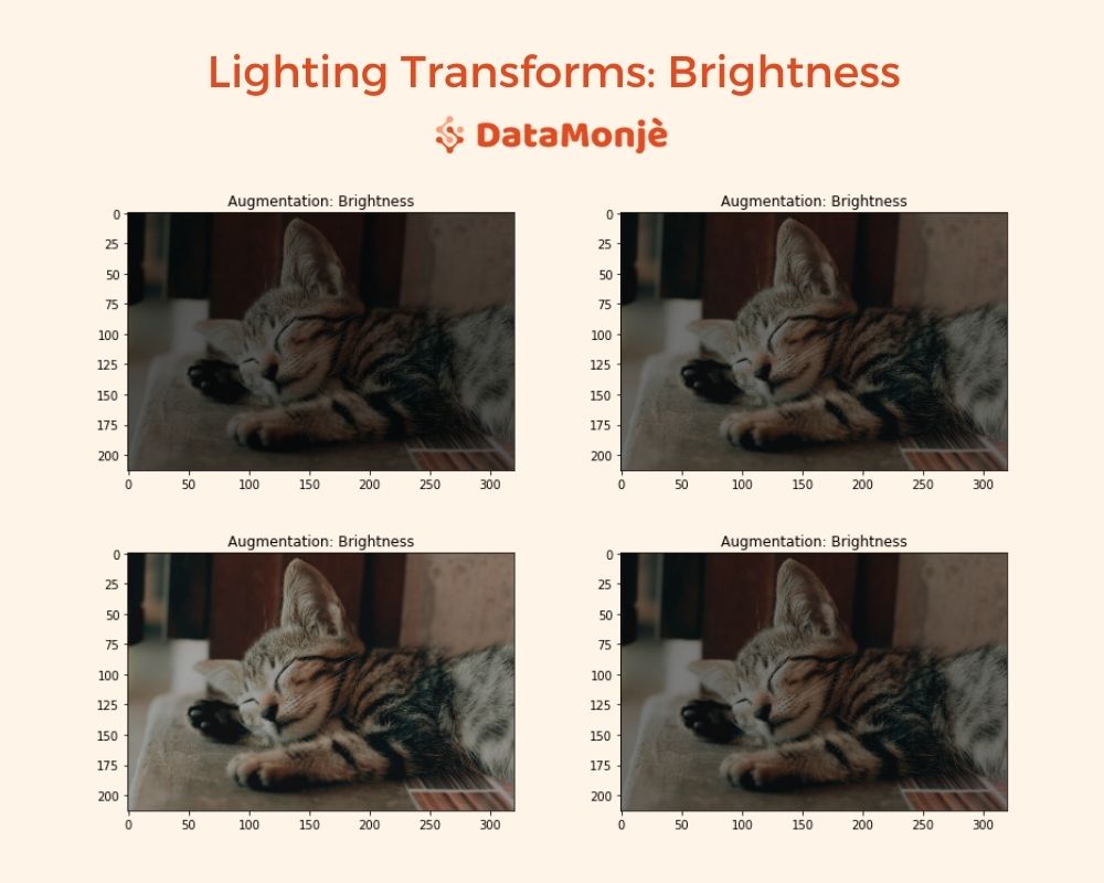
Lighting Transformations
This technique will change lighting conditions like brightness, contrast, saturation, etc. to augment a new image. These attributes are associated with lighting conditions like brightness is a measure of reflecting light.
We use lighting transformations to accommodate for the various lighting conditions at the time of an inference from a trained model.
Keras ImageDataGenerator class only provides augmentation for brightness with argument brightness_range which takes a tuple or a list of two floats specifying the brightness modification range.
If we set brightness_range = 0, the image will be all black and if we set that to 1, there won’t be any brightness changes.
image_augmentor = ImageDataGenerator(brightness_range=(0.3, 1))
data = image_augmentor.flow_from_directory(
    "/tmp/impath",
    target_size=(213, 320),
    batch_size=1,
)
pyplot.imshow(data.next()[0][0].astype('int'))
pyplot.title("Augmentation: Brightness")
Output:
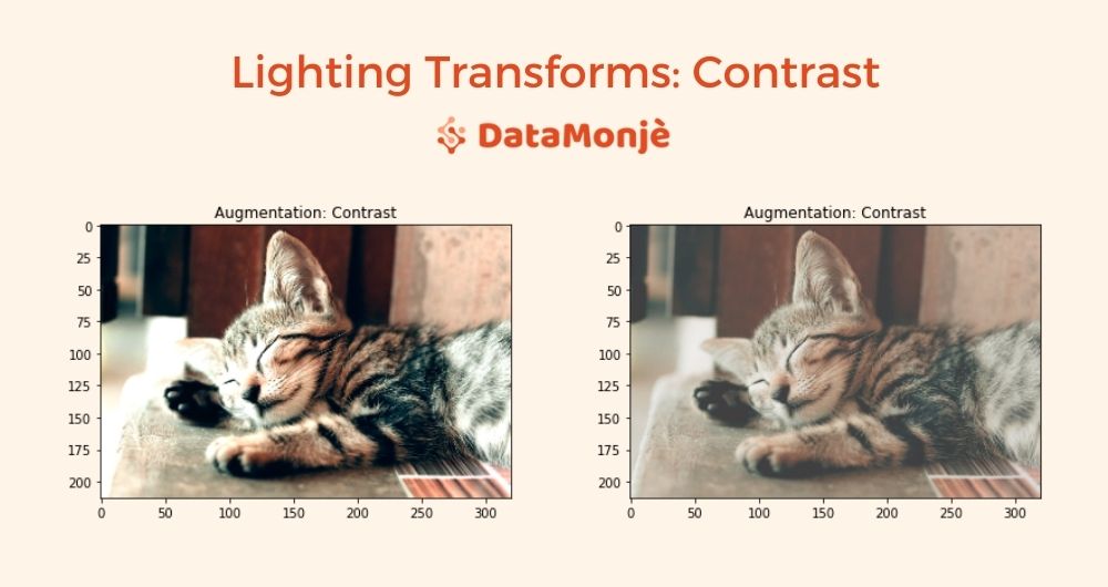
Custom Image Data Augmentation
As mentioned above, lightning transform is not only about brightness changes, it should also consider contrast, hue, and saturation transforms.
There is no default option for these transformations, we still can apply these manipulations using ImageDataGenerator’s preprocessing_function argument.
The preprocessing_function is a way to apply non-standard custom augmentation. It takes a defined function name as an argument.
This function is applied to each input once every default augmentation is applied including resize.
The function takes a numpy tensor of rank 3 as an input and outputs a numpy tensor of rank 3 as well.
Here is how we apply contrast, hue, and saturation using the preprocessing_function argument.
Let’s build a function for contrast first and then include it in ImageDataGenerator. Here we will use tensorflow.image module which provides out-of-the-box image processing functionalities.
Random Contrast
def custom_augmentation(np_tensor):

  def random_contrast(np_tensor):
    return tf.image.random_contrast(np_tensor, 0.5, 2)

  augmnted_tensor = random_contrast(np_tensor)
  return np.array(augmnted_tensor)
image_augmentor = ImageDataGenerator(preprocessing_function=custom_augmentation)
data = image_augmentor.flow_from_directory(
    "/tmp/impath",
    target_size=(213, 320),
    batch_size=1,
)
pyplot.imshow(data.next()[0][0].astype('int'))
pyplot.title("Augmentation: Contrast")
Output:
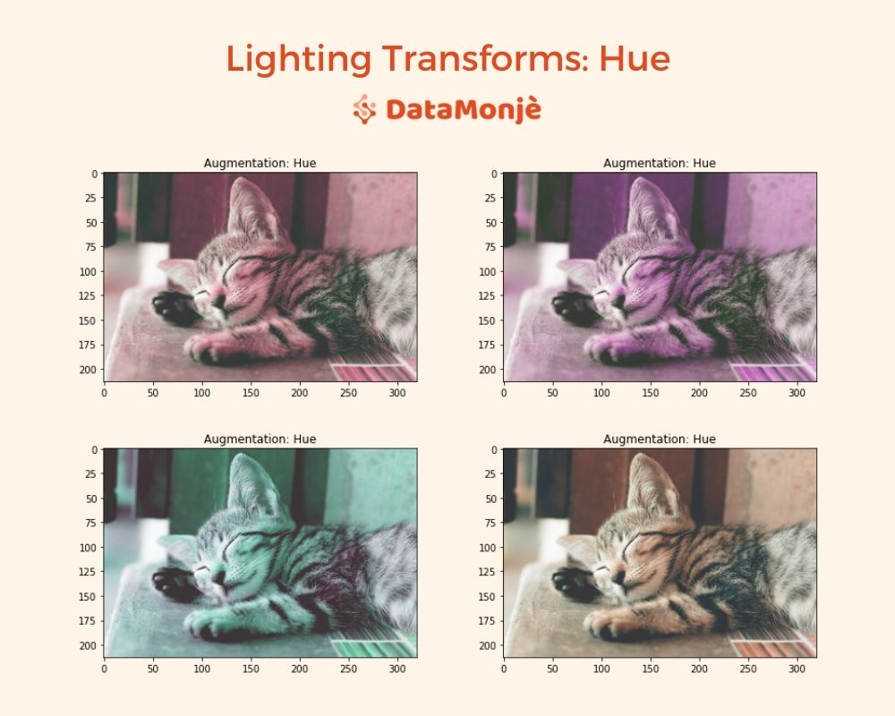
Random Hue
def custom_augmentation(np_tensor):

  def random_hue(np_tensor):
    return tf.image.random_hue(np_tensor, 0.5)

  augmnted_tensor = random_hue(np_tensor)
  return np.array(augmnted_tensor)
image_augmentor = ImageDataGenerator(preprocessing_function=custom_augmentation)
data = image_augmentor.flow_from_directory(
    "/tmp/impath",
    target_size=(213, 320),
    batch_size=1,
)
pyplot.imshow(data.next()[0][0].astype('int'))
pyplot.title("Augmentation: Hue")
Output:
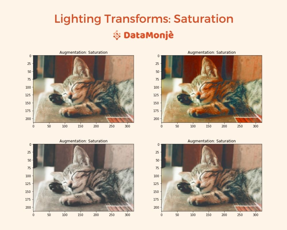
Random Saturation
def custom_augmentation(np_tensor):

  def random_saturation(np_tensor):
    return tf.image.random_saturation(np_tensor, 0.2, 3)

  augmnted_tensor = random_saturation(np_tensor)
  return np.array(augmnted_tensor)
image_augmentor = ImageDataGenerator(preprocessing_function=custom_augmentation)
data = image_augmentor.flow_from_directory(
    "/tmp/impath",
    target_size=(213, 320),
    batch_size=1,
)
pyplot.imshow(data.next()[0][0].astype('int'))
pyplot.title("Augmentation: Saturation")
Output:
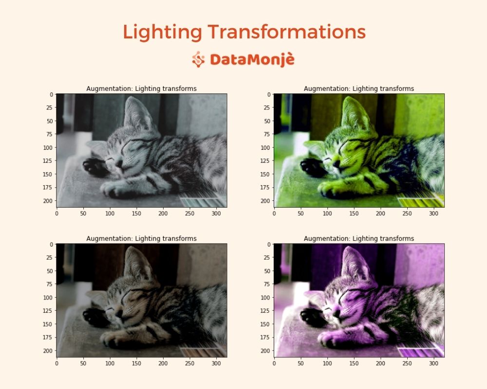
All lighting transformation together:
def custom_augmentation(np_tensor):

  def random_contrast(np_tensor):
    return tf.image.random_contrast(np_tensor, 0.5, 2)

  def random_hue(np_tensor):
    return tf.image.random_hue(np_tensor, 0.5)

  def random_saturation(np_tensor):
    return tf.image.random_saturation(np_tensor, 0.2, 3)

  augmnted_tensor = random_contrast(np_tensor)
  augmnted_tensor = random_hue(augmnted_tensor)
  augmnted_tensor = random_saturation(augmnted_tensor)
  return np.array(augmnted_tensor)

image_augmentor = ImageDataGenerator(brightness_range=(0.3, 1), \
                                     preprocessing_function=custom_augmentation)
data = image_augmentor.flow_from_directory(
    "/tmp/impath",
    target_size=(213, 320),
    batch_size=1,
)
pyplot.imshow(data.next()[0][0].astype('int'))
pyplot.title("Augmentation: Lighting transforms")
Output:
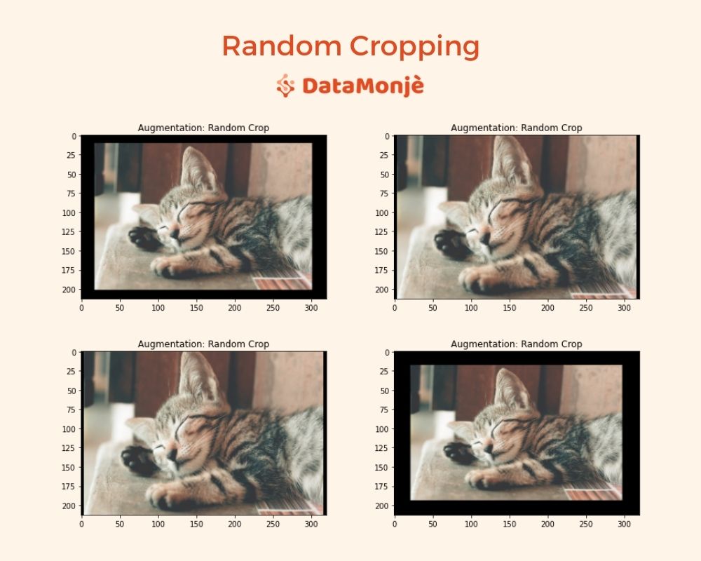
Random Cropping
The image cropping technique cut the original image to augment. The cropping area could be selected randomly or at the center.
Once an image is cropped, the processed image could be resized or could be padded based on requirements.
An image dataset, especially a small dataset, might have the class object at a particular location e.g. at the center, the random cropping could be useful in that case.
Even if that’s not the case, cropping would provide spatial variation that will help training for sure.
By default, ImageDataGenerator doesn’t provide this functionality. All following augmentations are not supported by default, but we can build a custom function to add on capabilities as we saw earlier.
def custom_augmentation(np_tensor):

  def random_crop(np_tensor):

    #cropped height between 70% to 130% of an original height
    new_height = int(np.random.uniform(0.7, 1.30) * np_tensor.shape[0])

    #cropped width between 70% to 130% of an original width
    new_width = int(np.random.uniform(0.7, 1.30) * np_tensor.shape[1])

    # resize to new height and width
    cropped = tf.image.resize_with_crop_or_pad(np_tensor, new_height, new_width)

    return tf.image.resize(cropped, np_tensor.shape[:2])

  augmnted_tensor = random_crop(np_tensor)
  return np.array(augmnted_tensor)

image_augmentor = ImageDataGenerator(preprocessing_function=custom_augmentation)
data = image_augmentor.flow_from_directory(
    "/tmp/impath",
    target_size=(213, 320),
    batch_size=1,
)
pyplot.imshow(data.next()[0][0].astype('int'))
pyplot.title("Augmentation: Random Crop")
Output:
Noise Addition
What we visually perceive as an image is fed as numbers to machine learning algorithms.
If we add or subtract a small number from an original image, visually we can’t even notice a difference but for algorithms, it's a big deal.
Adding such noise could break convolutional neural networks. Here is the example:
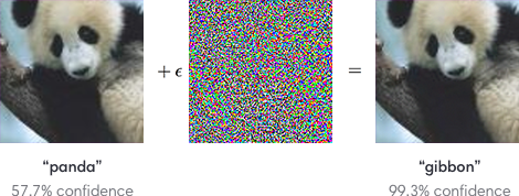
In addition to that such noise appears due to lighting conditions like a photo taken in low light conditions you would notice grains in the picture.
Adding a random noise won’t just work as augmentation but also as a preventive measure against adversarial attacks.
For that, we will create a random noise with a mean of 0 and a variance between 1 to 25 and add that to an original image.
def custom_augmentation(np_tensor):

  def gaussian_noise(np_tensor):
    mean = 0
    # variance: randomly between 1 to 25
    var = np.random.randint(1, 26)
    # sigma is square root of the variance value
    noise = np.random.normal(mean,var**0.5,np_tensor.shape)
    return np.clip(np_tensor + noise, 0, 255).astype('int')

  augmnted_tensor = gaussian_noise(np_tensor)
  return np.array(augmnted_tensor)

image_augmentor = ImageDataGenerator(preprocessing_function=custom_augmentation)
data = image_augmentor.flow_from_directory(
    "/tmp/impath",
    target_size=(213, 320),
    batch_size=1,
)
pyplot.imshow(data.next()[0][0].astype('int'))
pyplot.title("Augmentation: Random gaussian noise")
Here, the first image is output from our noise augmentation but you wouldn’t notice any significant difference.
The other three images are for illustration purposes only to develop a better understanding of noise addition. These images are created by adding Gaussian noise with variance values of 10, 50, and 100.
Output:
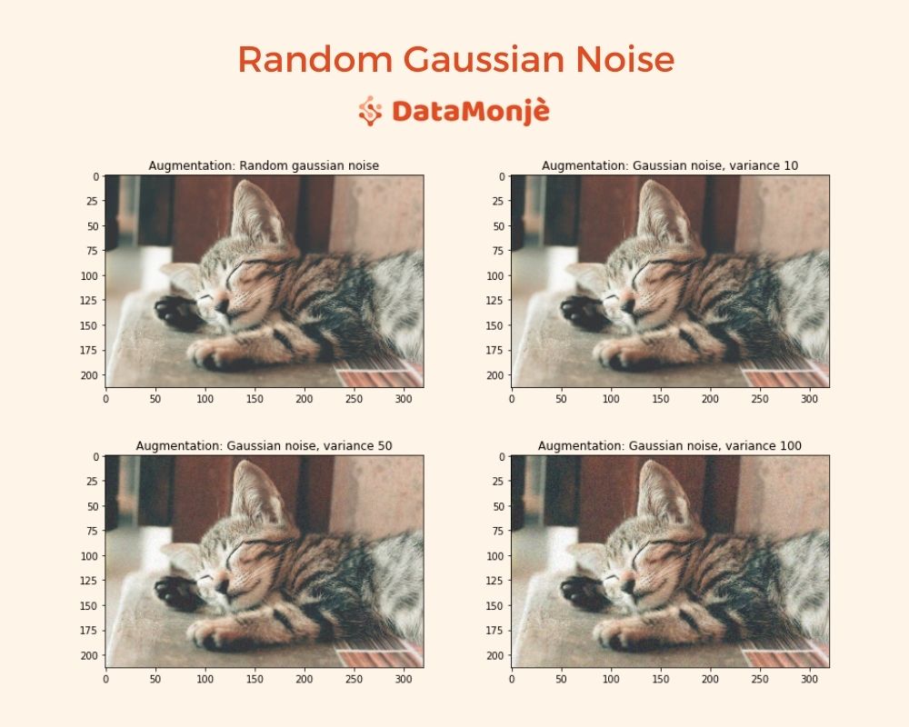
I bet, now you would be able to see the difference. As we increase variance, we see more and more noise being visible.
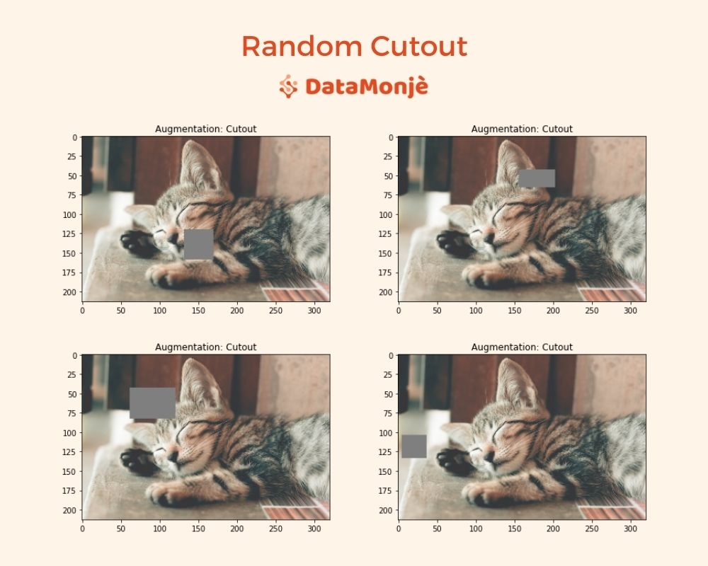
Random Image Cutout
The cutout augmentation cuts out a part of an image randomly. We do this by picking a portion of an image and setting pixel values for that part to a constant value like 0, 255, or 127 (or any other).
This is useful to make the algorithm not focus on certain features only for decision making.
For example, cats can be identified due to their ears, face, nose, etc., but if ears are properly visible in all training images, the algorithm will learn to classify an image to cat by seeing ears only.
Cutout decreases the dependency on the few most dominant features and helps to generalize better.
def custom_augmentation(np_tensor):

  def cutout(np_tensor):
    cutout_height = int(np.random.uniform(0.1, 0.2) * np_tensor.shape[0])
    cutout_width = int(np.random.uniform(0.1, 0.2) * np_tensor.shape[1])
    cutout_height_point = np.random.randint(np_tensor.shape[0]-cutout_height)
    cutout_width_point = np.random.randint(np_tensor.shape[1]-cutout_width)
    np_tensor[cutout_height_point:cutout_height_point+cutout_height, cutout_width_point:cutout_width_point+cutout_width, :] = 127
    return np_tensor

  augmnted_tensor = cutout(np_tensor)
  return np.array(augmnted_tensor)

image_augmentor = ImageDataGenerator(preprocessing_function=custom_augmentation)
data = image_augmentor.flow_from_directory(
    "/tmp/impath",
    target_size=(213, 320),
    batch_size=1,
)
pyplot.imshow(data.next()[0][0].astype('int'))
pyplot.title("Augmentation: Cutout")
Output:
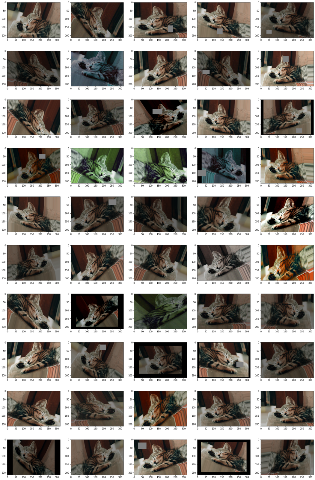
Putting All Augmentations Together
Here for custom augmentation, I used contrast, hue, and saturation with 10% probability, crop and noise with 20% probability, and cutout with 30% probability. Here is the result:
If you need to refer to the code for all these augmentations, you can download the jupyter notebook here.
Image Augmentation in an Action
In this section, we will explore how image augmentation affects training. To do so, we will work on cat vs dog classification. The dataset can be downloaded from here.
We will download and extract data. The directory structure would look like below.
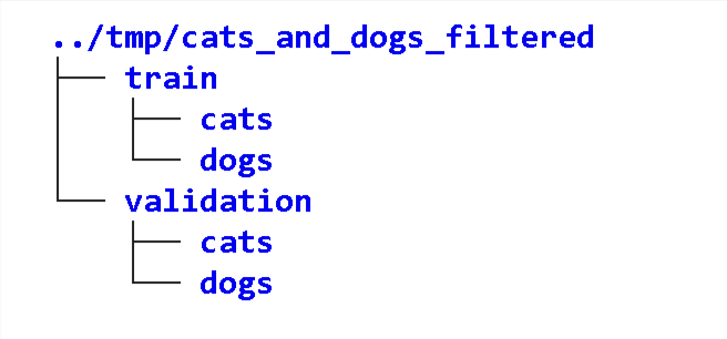
The cats and dogs are folders and contain associated images.
To have the first-hand experience, we will train a model first without augmentation and then with augmentation.
We will use a simple CNN architecture as we want to keep things simple, but the performance can be improved with state-of-the-art neural network architectures and transfer learning.
Here is the architecture we have used.
model = tf.keras.models.Sequential([

    tf.keras.layers.Conv2D(16, (3,3), activation='relu', input_shape=(150, 150, 3)),
    tf.keras.layers.MaxPooling2D(2,2),
    tf.keras.layers.Conv2D(32, (3,3), activation='relu'),
    tf.keras.layers.MaxPooling2D(2,2),
    tf.keras.layers.Conv2D(64, (3,3), activation='relu'),
    tf.keras.layers.MaxPooling2D(2,2),
    tf.keras.layers.Flatten(),
    tf.keras.layers.Dense(512, activation='relu'),
    tf.keras.layers.Dense(1, activation='sigmoid')
])
model.compile(optimizer=tf.keras.optimizers.Adam(),
              loss='binary_crossentropy',
              metrics = ['accuracy'])
Training without augmentation
train_datagen = ImageDataGenerator( rescale = 1.0/255. )
test_datagen  = ImageDataGenerator( rescale = 1.0/255. )

train_generator = train_datagen.flow_from_directory(train_dir,
                                                    batch_size=32,
                                                    class_mode='binary',
                                                    target_size=(150, 150))

validation_generator =  test_datagen.flow_from_directory(validation_dir,
                                                     batch_size=32,
                                                     class_mode  = 'binary',
                                                     target_size = (150, 150))

history1 = model.fit(train_generator,
                              validation_data=validation_generator,
                              steps_per_epoch=63,
                              epochs=25,
                              validation_steps=32,
                              verbose=1)

pyplot.plot(history1.history['accuracy'])
pyplot.plot(history1.history['val_accuracy'])
pyplot.title('Accuracy: Training without augmentation')
pyplot.ylabel('accuracy')
pyplot.xlabel('epoch')
pyplot.legend(['train', 'test'], loc='upper left')
pyplot.show()

pyplot.plot(history1.history['loss'])
pyplot.plot(history1.history['val_loss'])
pyplot.title('Loss: Training without augmentation')
pyplot.ylabel('loss')
pyplot.xlabel('epoch')
pyplot.legend(['train', 'test'], loc='upper left')
pyplot.show()
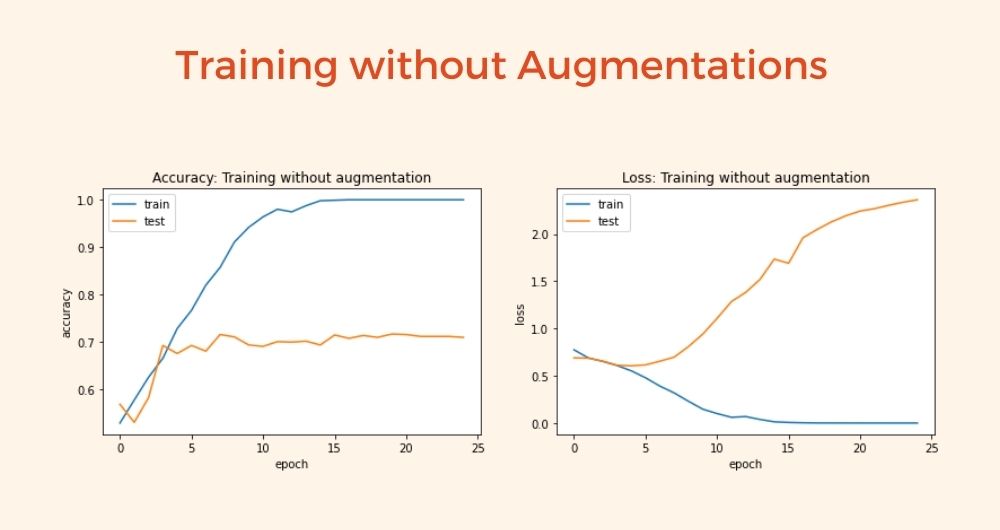
The accuracy and loss look like below:
Training with augmentation
train_datagen  = ImageDataGenerator(horizontal_flip=True,
                                     rotation_range = 30, brightness_range=[0.4, 0.99],
                                     width_shift_range = 0.1, height_shift_range = 0.1, zoom_range = [0.8, 1.25], shear_range= 30,
                                     preprocessing_function=custom_augmentation,
                                    rescale = 1.0/255. )
test_datagen  = ImageDataGenerator( rescale = 1.0/255. )

train_generator = train_datagen.flow_from_directory(train_dir,
                                                    batch_size=32,
                                                    class_mode='binary',
                                                    target_size=(150, 150))

validation_generator =  test_datagen.flow_from_directory(validation_dir,
                                                         batch_size=32,
                                                         class_mode  = 'binary',
                                                         target_size = (150, 150))
history2 = model.fit(train_generator,
                              validation_data=validation_generator,
                              steps_per_epoch=63,
                              epochs=25,
                              validation_steps=32,
                              verbose=2)
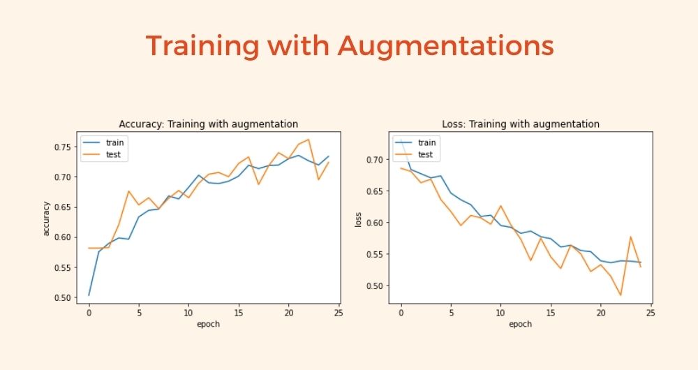
The accuracy and loss look like below for the model with augmentations:
We can see that without augmentation, we are facing overfitting and validation accuracy does not exceed 0.72.
On the other hand, with augmentation, there is no overfitting. Validation metrics are continuously moving with training metrics.
The validation accuracy is constantly improving. We would be able to achieve good performance if we train the model for a larger number of epochs.
Image Augmentation with Tensorflow Layers
You must be thinking that is ImageDataGenerator the only way for in-memory augmentation? Certainly not.
We can use neural network layers for image augmentation. The experimental preprocessing layers module from tensorflow.keras is useful here. Let’s directly dive into code as we know all the theories.
augmentation = tf.keras.Sequential([
  layers.experimental.preprocessing.RandomFlip("horizontal_and_vertical"),
  layers.experimental.preprocessing.RandomTranslation(0.2, 0.2),
  layers.experimental.preprocessing.RandomHeight(0.1),
  layers.experimental.preprocessing.RandomWidth(0.1),
  layers.experimental.preprocessing.RandomZoom(0.25),
  layers.experimental.preprocessing.RandomRotation(0.2),
  layers.experimental.preprocessing.RandomContrast(0.5),
  layers.experimental.preprocessing.Resizing(213, 320)
])

plt.figure(figsize=(15, 10))
for i in range(9):
  augmented_image = augmentation(data.next()[0])
  ax = plt.subplot(3, 3, i + 1)
  plt.imshow(np.array(augmented_image[0]).astype('int'))
Output:

Building Custom Augmentation Layers
Cool, right? But only limited image augmentation layers exist. What if we want custom augmentation as we did with the ImageDataGenerator class.
There is a way, you can always build a custom layer as per your requirements. In the below example, we added random saturation capability with a custom layer.
class RandomSaturation(tf.keras.layers.Layer):
    def __init__(self, saturation_range=[0.5, 1.5], clip_value=1, **kwargs):
        super(RandomSaturation, self).__init__(**kwargs)
        self.lower_range = saturation_range[0]
        self.upper_range = saturation_range[1]
        self.clip_value = clip_value

    def call(self, images, training=None):
        if not training:
            return images

        images = tf.image.random_saturation(images, self.lower_range, self.upper_range)
        images = tf.clip_by_value(images, 0, self.clip_value)
        return images

sat_layer = RandomSaturation ([0.2, 3], clip_value=255)
saturated_image = sat_layer(data.next()[0], training=True)
plt.imshow(np.array(saturated_image)[0].astype('int'))
plt.title("Image saturation with custom layer")
Output:

We can combine custom and in-built layers for image augmentation. Below is how you can define model with this approach:
train_datagen = ImageDataGenerator( rescale = 1.0/255. )
test_datagen  = ImageDataGenerator( rescale = 1.0/255. )

train_generator = train_datagen.flow_from_directory(train_dir,
                                                    batch_size=32,
                                                    class_mode='binary',
                                                    target_size=(150, 150))

validation_generator =  test_datagen.flow_from_directory(validation_dir,
                                                         batch_size=32,
                                                         class_mode  = 'binary',
                                                         target_size = (150, 150))

model = tf.keras.models.Sequential([
    layers.experimental.preprocessing.RandomFlip("horizontal_and_vertical"),
    layers.experimental.preprocessing.RandomTranslation(0.2, 0.2),
    layers.experimental.preprocessing.RandomHeight(0.1),
    layers.experimental.preprocessing.RandomWidth(0.1),
    layers.experimental.preprocessing.RandomZoom(0.25),
    RandomSaturation ([0.2, 3]),
    layers.experimental.preprocessing.RandomRotation(0.2),
    layers.experimental.preprocessing.RandomContrast(0.5),
    layers.experimental.preprocessing.Resizing(150, 150),
    layers.Conv2D(16, (3,3), activation='relu', input_shape=(150, 150, 3)),
    layers.MaxPooling2D(2,2),
    layers.Conv2D(32, (3,3), activation='relu'),
    layers.MaxPooling2D(2,2),
    layers.Conv2D(64, (3,3), activation='relu'),
    layers.MaxPooling2D(2,2),
    layers.Flatten(),
    layers.Dense(512, activation='relu'),
    layers.Dense(1, activation='sigmoid')
])
Once we build the model as shown above, we can compile and train the model as we do with any other model.
Till now, we have seen in-memory image augmentation using Keras and tensorflow.
We used ImageDataGenerator and augmentation layers along with customization for greater flexibility.
If you are looking for an image data augmentation using fastai, I would recommend taking a look at this brilliant Kaggle notebook.
Where do you go from here?
Get your hands dirty
I have created a jupyter notebook that consists of all the code mentioned here.
It would be a great start to run that code by yourself and play around with the parameters to have a fundamental understanding of what each augmentation does and how it affects the end result.
And once you get comfortable, try implementing a custom augmentation using pre pre-process function or a custom layer. One such augmentation example is image blur.
Download the jupyter notebook
Ask questions
Once you start with this code, you might have questions.
I would encourage you to ask questions in the comment section, I would do my best to answer your concerns.
Anand is a marketer turned data scientist. He is mostly interested in the current and future state of artificial intelligence and loves to write about topics related to machine learning and deep learning.
Hello Anand Borad, thank you about it, very good post.
how can i count images that have increased in my dataset after using augmentation with Tensorflow Layers?