A Beginner’s Guide to Loss functions for Regression Algorithms

Loss function in supervised machine learning is like a compass that gives algorithms a sense of direction while learning parameters or weights.

This blog will explain the What? Why? How? and When? to use Loss Functions including the mathematical intuition behind that. So without wasting further time, Let’s dive into the concepts.

What is Loss Function?

Every supervised learning algorithm is trained to learn a prediction. These predictions should be as close as possible to label value / ground-truth value. The loss function measures how near or far are these predicted values compared to original label values.

Loss functions are also referred to as error functions as it gives an idea about prediction error.

Loss Functions, in simple terms, are nothing but an equation that gives the error between the actual value and the predicted value.

The simplest solution is to use a difference between actual values and predicted values as an error, but that’s not the case. Academicians, researchers, or engineers don’t use this simple approach.

For an example of a Linear Regression Algorithm, the squared error is used as a loss function to determine how well the algorithm fits your data.

But why not just the difference as error function?

The intuition is if you take just a difference as an error, the sign of the difference will hinder the model performance. For example, if a data point has an error of 2 and another data point has an error of -2, the overall difference will be zero, but that’s wrong.

Another solution that we might come up with is instead of taking the signed difference, we could use unsigned difference, e.g. we use MOD, |x|. The unsigned difference is called an Absolute Error. This could work in some cases but not always.

But again, why can’t we use the absolute error metric for all cases? why do we have different types of Loss functions? To answer those questions, let’s dive into the types of Loss Functions and What? Why? How? and When? of it.

Types of loss functions

Researchers are studying Loss Functions over the years for perfect loss functions which can be fit for all.

During this process, many loss functions have emerged. Broadly LFs can be classified into two types.

• Loss Functions for Regression Tasks
• Loss Functions for Classifications Tasks

In this article, we will focus on loss functions for regression algorithms and will cover classification algorithms in another article.

Loss Functions for Regression

We will discuss the widely used loss functions for regression algorithms to get a good understanding of loss function concepts.

Algorithms like Linear Regression, Decision Tree, Neural networks, majorly use the below functions for regression problems.

• Mean Squared Loss(Error)
• Mean Absolute Loss(Error)
• Huber Loss

Mean Squared Error

Mean squared error (MSE) can be computed by taking the actual value and predicted value as the inputs and returning the error via the below equation (mean squared error equation).

Here N is the number of training samples, yi is the actual value of the ith sample, and yi_hat is the predicted value of the corresponding sample. This Equation gives the mean of the square of the difference.

Mean Squared Error is most commonly used as it is easily differentiable and has a stable nature.

Why Mean Squared Error?

As we have seen, the equation is very simple and thus can be implemented easily as a computer program. Besides that, it is powerful enough to solve complex problems.

The equation we have is differentiable hence the optimization becomes easy. This is one of the reasons for adopting MSE widely. Let’s build intuition mathematically with an assumption that you are familiar with calculus.

The below is the general equation for the differentiation of x^n:

This implies for n=2 (squared error), the equation will be:

Comparing this standard differentiation formula to MSE with removing the normalization part (which is computing the mean) and the summation part (we can ignore the mean and summation for simplicity), the result will be:

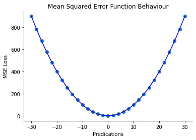
Here is what it looks like when we plot a graph of MSE loss against a signed difference between the actual value and the predicted value.

When to use MSE?

Mean Squared Error is preferred to use when there are low outliers in the data. This is one of the drawbacks of MSE.

As the MSE loss uses a square of a difference, the loss will be huge for outliers and it adversely affects the optimized solution. Using standardized data is efficient for better optimization using this loss.

Advantages

• Simple Equation, Can be optimizedg easily compared to other equations.
• Has proven its ability over the years, this is majorly used in fields like signal processing

Disadvantages

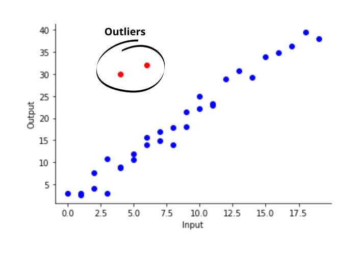
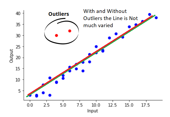
• It is highly affected by Outliers. So if the data contains outliers, better not to use it.

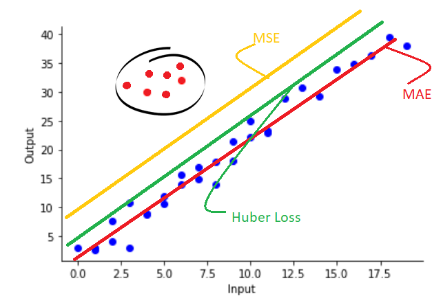
Outliers refer to the data that does not follow the same pattern(trend) as most data are following. The below graph shows a clear explanation of this:

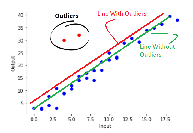
The linear regression line with MSE loss will tend to align with those outliers.

How to implement MSE loss?

How can we compute programmatically? Below is the Python Code for realizing the Mean Squared Loss Function. The Code can be as simple as this:

    
import numpy as np

actual = np.random.randint(0, 10, 10)
predicted = np.random.randint(0, 10, 10)

print('Actual :', actual)
print('Predicted :', predicted)

ans = []

# The Computation through applying Equation 
for i in range(len(actual)):
    ans.append((actual[i]-predicted[i])**2)

MSE = 1/len(ans) * sum(ans)
print("Mean Squared error is :", MSE)

# OUTPUTS #
# Actual : [2 1 6 3 8 2 2 3 9 8]
# Predicted : [2 0 9 5 7 6 3 6 5 4]
# Mean Squared error is : 7.300000000000001
    

 The shape (dimensions) of the two arrays (Actual and Predicted) must be the same. The above code can be generalized for n-dim as below:

    
import numpy as np

actual = np.random.randint(0, 10, (4,10))
predicted = np.random.randint(0, 10, (4,10))

print('actual :', actual)
print('predicted :', predicted)

# ans = np.subtract(actual, predicted)
# ans_sq = np.square(ans)
# MSE = ans_sq.mean()
# or

MSE = np.square(np.subtract(actual, predicted)).mean()
print("Mean Squared error is :", MSE)

# OUTPUT #
'''
actual : [[2 9 1 0 2 3 4 3 8 7]
 [7 6 3 9 4 0 0 3 8 5]
 [7 1 8 3 7 1 4 4 1 0]
 [3 3 4 6 1 7 5 1 5 7]]
predicted : [[1 4 0 0 2 7 6 4 4 3]
 [4 8 3 6 2 8 7 9 9 6]
 [8 9 8 3 3 2 6 3 0 7]
 [4 2 2 2 6 4 9 2 3 6]]
Mean Squared error is : 11.8
'''
    

Mean Absolute Error

Similar to MSE, Mean Absolute Error (MAE) gives you how far/close are you from the prediction value, but the twist is here instead of squaring you will be performing the mod operation. Mathematically it can be written as

Here N is the number of training samples. yi is the actual label and yi_hat is the predicted output for ith sample/datapoint.

Why Mean Absolute Error?

This function is fairly simple and yet it works pretty well with outliers. It reduces the impact of outliers on final optimization.

Although, the problem lies in the differentiation of the equation. The optimization of the MAE function is a little bit tricky because of the Mod function. Let’s understand it mathematically to get the intuition.

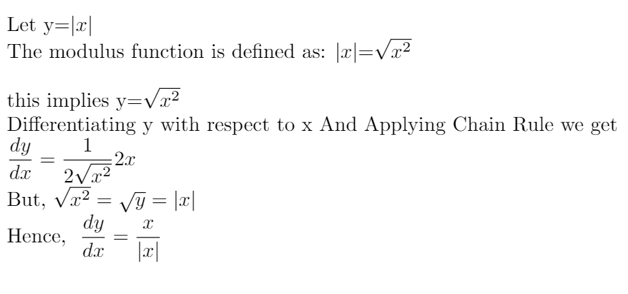
The below is the simple method for the differentiation of |x|:

If we compare this to the MAE equation, we get:

For positive (y-y_hat) values, the derivative is +1 and negative (y-y_hat) values, the derivative is -1.

The arises when y and y_hat have the same values. For this scenario (y-y_hat) becomes zero and derivative becomes undefined as at y=y_hat the equation will be non-differentiable! 

To avoid such conditions we can add a small epsilon value to the denominator so that the denominator will not become zero. The sample graph of the MAE function behavior is given below:

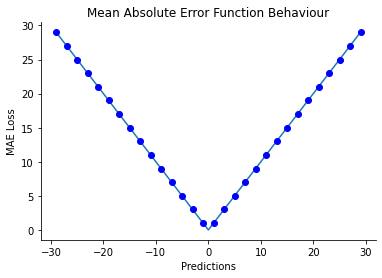
When to use Mean Absolute Error?

MAE is preferred to use when there is a chance of having outliers in the data. This is one of the Advantages of MAE. Using standardized data is efficient for better optimization using this loss.

Advantages

• It is not much affected by outliers. So if the data contains outliers, better to use MAE over MSE as the loss function.

Disadvantages

• The Optimization is a little bit complex compared to MSE

The drawback is if there are more data with irregular patterns (which may not be an outlier and might be useful data), the MAE will ignore those as well. The below figure shows this:

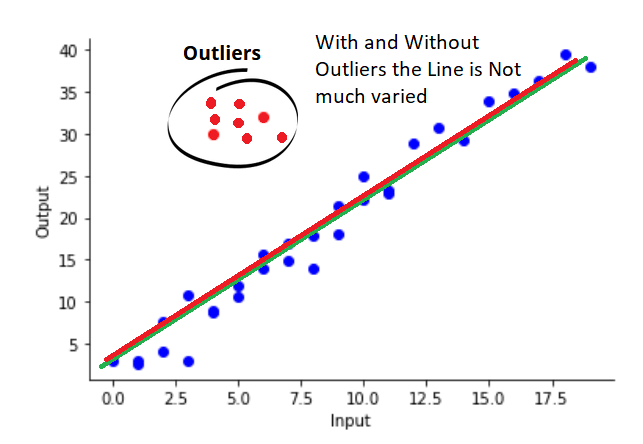
This is due to fact that MAE will penalize the algorithm based on the difference only (unlike the square of the difference in MSE). In that case, as more and more data fits into a pattern, it tends to ignore rare patterns.

How to implement MAE?

Now let’s get our hands dirty and code the MAE loss function. Here is the python code for the mean absolute error.

    
import numpy as np

actual = np.random.randint(0, 10, 10)
predicted = np.random.randint(0, 10, 10)

print('Actual :', actual)
print('Predicted :', predicted)

ans = []

# The Computation through applying Equation 
for i in range(len(actual)):
    ans.append((actual[i]-predicted[i])**2)

MAE = 1/len(ans) * sum(ans)
print("Mean Absolute error is :", MAE)
# OUTPUT #
Actual : [2 1 2 9 2 9 0 9 0 0]
Predicted : [9 6 6 8 1 4 8 1 4 9]
Mean Absolute error is : 5.2
    

For a one-dimensional space, the above code works fine, but for n-dimensional space, we need to use an optimized approach. we can program such efficient code using numpy easily.

    
import numpy as np

actual = np.random.randint(0, 10, (4,10))
predicted = np.random.randint(0, 10, (4,10))

print('actual :', actual)
print('predicted :', predicted)

MAE = np.abs(np.subtract(actual, predicted)).mean()
print("Mean Absolute error is :", MAE)

'''
# OUTPUT #
actual : [[7 8 3 0 9 2 9 5 5 0]
 [9 3 5 6 8 8 5 5 9 3]
 [0 9 4 7 7 7 8 4 1 6]
 [3 9 5 2 2 7 2 5 3 8]]
predicted : [[7 3 5 0 4 1 9 5 1 9]
 [5 2 4 0 7 7 1 2 5 1]
 [9 3 2 5 4 4 2 3 5 1]
 [8 9 1 6 0 9 3 6 2 7]]
Mean Absolute error is : 2.875
'''
    

Relevant Article

Guide to Image Data Augmentation: from Beginners to Advanced

Huber Loss

Huber Loss can be interpreted as a combination of the Mean squared loss function and Mean Absolute Error. The equation is:

Huber loss brings the best of both MSE and MAE.

The δ term is a hyper-parameter for Hinge Loss. The loss will become squared loss if the difference between y and y_hat is less than δ and loss will become a variation of an absolute error for y-y_hat > δ.

The intuition is to use an absolute error when the difference between the actual value and the predicted value is small and use the squared loss for larger error to enforce a high penalty to decrease the impact of outliers.

Why hinge loss?

Mean Squared Error and Mean Absolute Error both have their own advantages and disadvantages.

The Hinge loss tries to overcome the disadvantages by combining the goodness of both with the above equation.

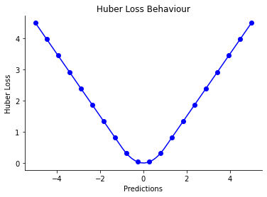
The below graph shows Huber loss vs prediction error. There is no sharp edge, instead, it has a smooth curve. A sharp edge means the function is not continuous at that point. A function has to be continuous to be differentiable.

This might make more sense once you see the code, we will clarify more in the implementation section.

When to use huber loss?

Huber loss can be useful when we need the balance of Mean squared error and mean absolute error.

The MAE will completely ignore the outliers (even if it contains 20–30% of data), but Huber loss can prevent the outliers to some extent, but if the outliers are large it will make a balance.

The below figure clearly explains this:

Advantages

• The Huber loss is effective when there are Outliers in data
• The optimization is easy, as there are no non-differentiable points

Disadvantages

• The equation is a bit complex and we also need to adjust the δ based on our requirement

How to implement huber loss?

Below is the python implementation for Huber loss.

Here we are taking a mean over the total number of samples once we calculate the loss (have a look at the code). It’s like multiplying the final result by 1/N where N is the total number of samples. This is standard practice.

The function calculates both MSE and MAE but we use those values conditionally. If the condition (|y-y_pred| ≤ δ (delta)) then it uses MSE else MAE loss is used.

    
import numpy as np

def huber_loss(y_pred, y, delta=1):
    huber_mse = 0.5*np.square(np.subtract(y,y_pred))
    huber_mae = delta * (np.abs(np.subtract(y,y_pred)) - 0.5 * delta)
    return np.where(np.abs(np.subtract(y,y_pred)) <= delta, huber_mse, huber_mae).mean()

actual = np.random.randint(0, 10, (2,10))
predicted = np.random.randint(0, 10, (2,10))

print('actual :', actual)
print('predicted :', predicted)
print("Mean Absolute error is :", huber_loss(actual, predicted))
    

As we have discussed the major three functions, you must have realized that the higher the adaptive nature, the more accurate prediction it can make.

Researchers have invented and explored several loss functions. Their major aim is to find a loss function that can solve based on data (Adaptive).

As a beginner, these losses are more than enough, but if you still want to dig deeper and explore more loss functions, I highly recommend you to go through Charbonnier loss, pseudo-Huber loss, and generalized Charbonnier loss functions.

Cool! We have finished the Loss Functions for Regression part. In the next part, I will cover the loss functions for Classification.

Navaneeth Sharma

Navaneeth Sharma is a content contributor at DataMonje. He is passionate about Artificial intelligence. Navaneeth has contributed to publishing two machine learning integrated pip packages Scrapegoat and AksharaJaana. He aims to become a full-time AI Research Engineer.