A Beginner’s Guide to Loss functions for Classification Algorithms

Welcome to the second part of the Complete Guide to Loss Functions. Previously we had studied the Regression Losses in depth. In this blog, we will go through the details of the Classification Loss Functions.

Classification algorithms like Logistic Regression, SVM (Support Vector Machines), Neural Networks use a specific set of loss functions for the weights to learn. As the Regression losses were very intuitive, the classification loss functions involve slight complexity. The following are the set of popular loss functions for classification.

• Binary Cross-Entropy Loss
• Multi-class Cross-Entropy Loss (Categorical Cross-Entropy)
• Hinge Loss

Without wasting further time, let’s dive in.

Binary Cross-Entropy Loss

Cross-Entropy is a measure of loss between two probability distributions. What does that mean now? Entropy is a measure of randomness. For example, if we consider three containers with solid, liquid, and gas. The entropies would be E(gas)>E(liquid)>E(solid). So as much data is random, the entropy would be higher. Now Cross-Entropy is just the difference between two or more entropies. 

Binary Cross-entropy is a loss for the classification problems which has two categories or classes. The equation can be given by

Here, N is the total number of samples or data points. y is the expected output, y_hat is the predicted output. But wait, Can’t we use metrics like MSE or MAE for the classification? Let’s see why we need loss like cross-entropy.

Why cross entropy loss?

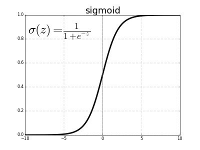
Let’s take an example to understand the need. For binary classification, usually, the sigmoid function is used as the output function. Sigmoid will squash the input to between 0 and 1. Thus the output will look like probability or percentage.

Let’s understand this with an example. Assume that the expected output is 0 and prediction is 0.9.

The prediction must be near 0 if the algorithm is trained properly. Instead, it gave 0.9 as output which is far away from the ground truth value as output can only take values between 0 and 1.

This means the loss value should be high for such prediction in order to train better.

Here, if we use MSE as a loss function, the loss = (0 – 0.9)^2 = 0.81

While the cross-entropy loss =  -(0 * log(0.9) + (1-0) * log(1-0.9)) = 2.30 

On other hand, values of the gradient for both loss function makes a huge difference in such a scenario. In this case gradient for MSE is -1.8 and cross-entropy is -10.

Ignoring the sign (it indicates the direction), the magnitude of Cross-Entropy is much higher than MSE, which means it penalizes the error better for categories from MSE.

This is one of the reasons for choosing Categorical Cross Entropy as the loss for classification. As the function uses logarithms, it is also known as log loss. The graph for Cross-Entropy loss or Log Loss can be given as

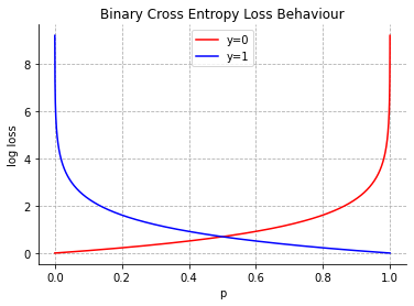
The above graph will help you to understand very intuitively how binary cross-entropy loss behaves.

If we consider y=0 as the expected output, the log loss is less for small values, and as the p (predicted value of y by algorithm) increases, the log loss increases rapidly.

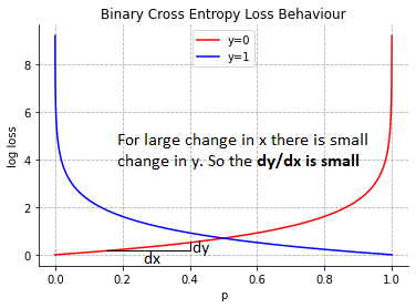
As most algorithms are dependent upon the gradient. Let’s dig deep there. For small values of p, the gradients are small.

For larger values of p, the gradients are high.

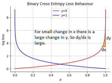
If the algorithm is predicting wrongly by giving the high value of probability, the loss function must penalize it. This is exactly what log loss is doing.

When and how to use binary cross-entropy loss?

Binary Cross-Entropy loss is usually used in binary classification problems with two classes. The Logistic Regression, Neural Networks use binary cross-entropy loss for 2 class classification problems.

The following is the code for Binary cross-entropy in python.

    
import numpy as np

def log_loss(y_pred, y):
    return -(np.multiply(y,np.log(y_pred)) + np.multiply(1-y,np.log(1-y_pred)))
 
actual = np.linspace(0,1,12)
predicted = np.asarray([0,1,0,0,1,1,1,0,1,1])
 
l_loss = log_loss(actual[1:-1], predicted)
 
print('actual :', actual[1:-1])
print('predicted :', predicted)
 
print("Log Loss:", l_loss)

# OUTPUTS #
# actual : [0.09 0.18 0.27 0.36 0.45 0.54 0.63 0.72 0.81 0.90]
# predicted : [0 1 0 0 1 1 1 0 1 1]
# Log Loss: [0.09531018 1.70474809 0.31845373 0.45198512 0.78845736 0.6061358 0.45198512 1.29928298 0.2006707  0.09531018]
    

Categorical Cross-Entropy

Categorical cross-entropy is just an extension of binary cross-entropy. This loss function is used extensively in neural networks for multi-class classification problem statements. The general equation is given by 

Let’s understand through this perspective. 

Consider we have five animal categories to predict: Horse, Cat, Dog, Lion, and Cheetah.

At first, the last layer of the neural network gives an array of numbers as an output. Then the output is transformed between zero and one using output squash function – Softmax (just like we need sigmoid for binary cross-entropy, we need softmax for categorical cross-entropy), such that the sum of all the output is equal to 1. The softmax equation is given by

The following diagram shows the above explanation

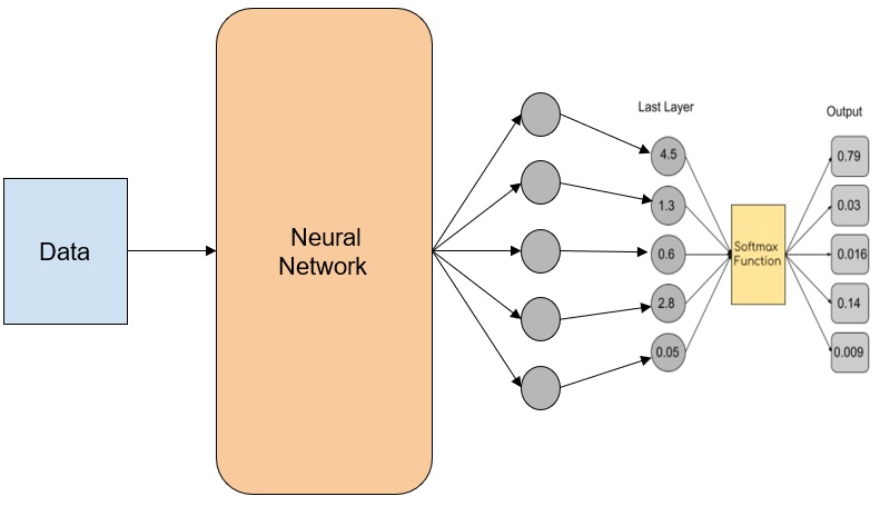
If the actual data sample is of a dog, the output we got is wrong because 79% probability is predicted as a horse.

So, the loss function needs to correct and give an array (comparing the one-hot encoding vector) so that the neural network can backpropagate and learn the correct label. The categorical cross-entropy solves this problem (the code takes the same example).

For multi-class classification problems, the categorical cross-entropy loss function plays a crucial role in deep learning algorithms because the loss can penalize the class that needs to be corrected.

The explanation of the equation is similar to the binary cross-entropy but mapping it to higher dimensions.

The below is the python code for categorical cross entropy.

    
import numpy as np
def crossEntropy(y_pred, y):
    ce_loss = np.multiply(y,np.log(y_pred))
    return -np.sum(ce_loss)
 
o_layer = np.array([0.79, 0.03, 0.016, 0.14, 0.009])
actual = np.array([0,0,1,0,0])

print("Output layer values:", o_layer)
print("One-Hot Encoded values:", actual)

print("Cross Entropy loss:", crossEntropy(o_layer, actual))

# Output
# Output layer values: [0.79  0.03  0.016 0.14  0.009]
# One-Hot Encoded values: [0 0 1 0 0]
# Cross Entropy loss: 20.67
   

Relevant Article

Guide to Image Data Augmentation: from Beginners to Advanced

Hinge Loss

Hinge Loss is a specific loss function used by Support Vector Machines (SVM). This loss function will help SVM to make a decision boundary with a certain margin distance.

SVM uses this loss function for figuring out the best possible decision boundary with margin. The Hinge loss actually arises from the constraints we are imposing on SVM. The equation for the loss is

Here, y is the actual outcome (either 1 or -1), and y_hat is the output of the classifier.

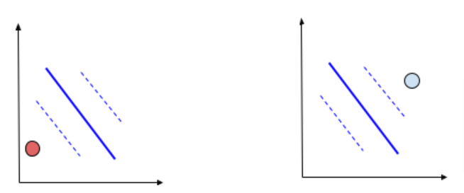
Diagrammatically the SVM can look like below:

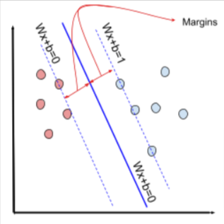
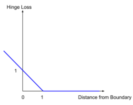
The hinge loss helps SVM to find optimized hyperplanes such that the margins are maximized. The graph of hinge loss is looks like:

Why does Hinge Loss work effectively?

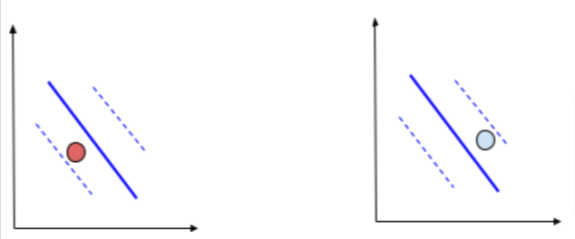
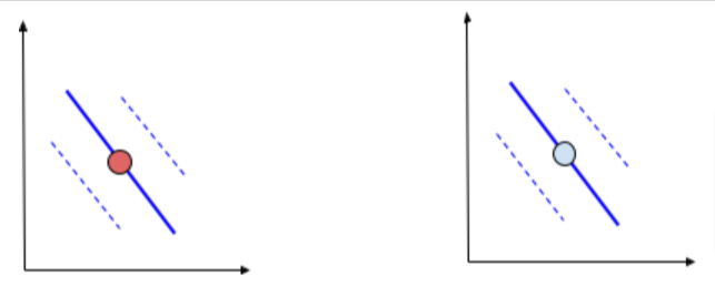
Consider the below data with decision boundary and margins, The points are linearly separable or we can separate via a line. The hinge loss can be explained in three stages. 

1. Points far from the margin
2. Points inside the margin but not in contact with the decision boundary
3. Points with contact of the decision boundary

The Points which are far from the decision boundary and away from the margin are easily separable by the hinge loss. The hinge loss for these data points which lie on the correct side will be zero. If it lies on the wrong side the loss will be very high.

The points which lie between the margin and the boundary will have some loss even though they are correctly classified. The loss will be between zero to one. This ensures the SVM separates well.

If the points lie on the decision boundary, those points will be penalized with a loss of 0.5.

The below is the python code for Hinge Loss.

    
import numpy as np

y = np.array([1,1,1,-1,-1,-1])
y_hat = np.array([0.5,3,5,2,-7,-9])
 
def hingeLoss(y, y_hat):
    return np.maximum(0, 1-y*y_hat)
 
print("Actual values:", y)
print("Distance from boundary with direction(sign):", y_hat)
 
print("Hinge Loss:", hingeLoss(y,y_hat))

# OUTPUTS #
# Actual values: [ 1  1  1 -1 -1 -1]
# Distance from boundary with direction(sign): [ 0.5  3.   5.   2.  -7.  -9. ]
# Hinge Loss: [0.5 0.  0.  3.  0.  0. ]
    

If the actual label is -1 and if the point is classified into +1 distance will be +ve, and the loss for that will be high (Actual: -1, Distance: 2, Loss: 3)

Amazing! We have finished the popular loss functions for Machine Learning! 

If you have any questions, kindly let me know in the comment below. I will try my best to resolve your doubt.

Navaneeth Sharma

Navaneeth Sharma is a content contributor at DataMonje. He is passionate about Artificial intelligence. Navaneeth has contributed to publishing two machine learning integrated pip packages Scrapegoat and AksharaJaana. He aims to become a full-time AI Research Engineer.