In-Depth Explanation to Gradient Descent: Working Principle and its Variants

A complete guide towards understanding Gradient Descent and its variants.

One of the core ideas of machine learning is that it learns via optimization. Gradient descent is an optimization algorithm that learns iteratively.

Here gradient refers to the small change, and descent refers to rolling down. The idea is, the error or loss will roll down with small steps, eventually reaching the minimum loss. The animation below shows it clearly.

Let’s understand the gradient descent algorithm via mathematical perspective and examples.

The simplest way to understand the gradient descent is by considering the linear regression with the mean squared loss function. Mathematically, gradient descent is

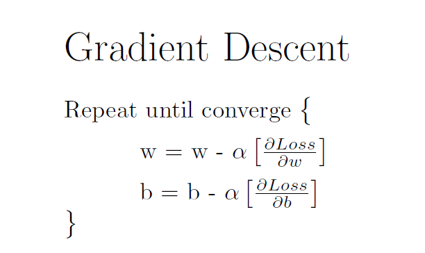
Here the w is the weight matrix, b is the bias matrix. Since the loss is mean squared error, the partial derivatives to w,b are

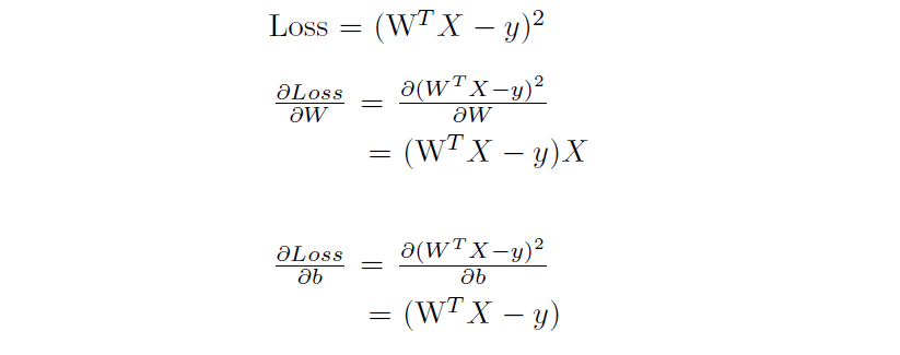
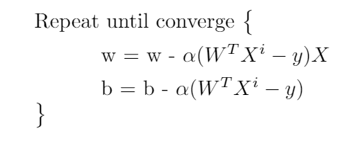
Now substituting the partial derivatives back to the gradient descent equation, we get

W and b are updated iteratively. The gradient descent needs an alpha term (known as the learning rate or steps). This term will be responsible for how fast the learning can happen. The alpha needs to be chosen appropriately.

If alpha is high, the loss may not converge or will not minimize. If alpha is too small, the convergence will happen but, the iterations taken to coverage will be high. The below animations will explain this more precisely.

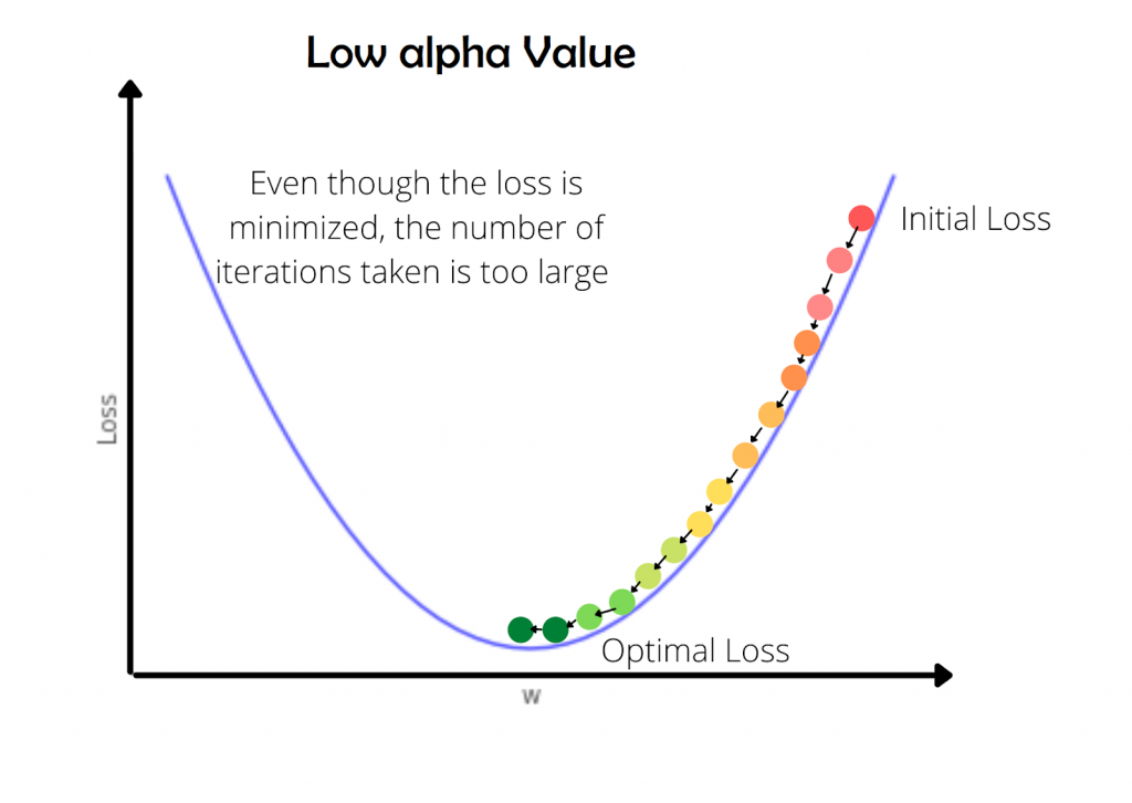
gradient descent with small learning rate

The low value of alpha is usually less than 10-6. This is crucial during deep learning since the model consumes more time to train. So, the learning needs to be faster.

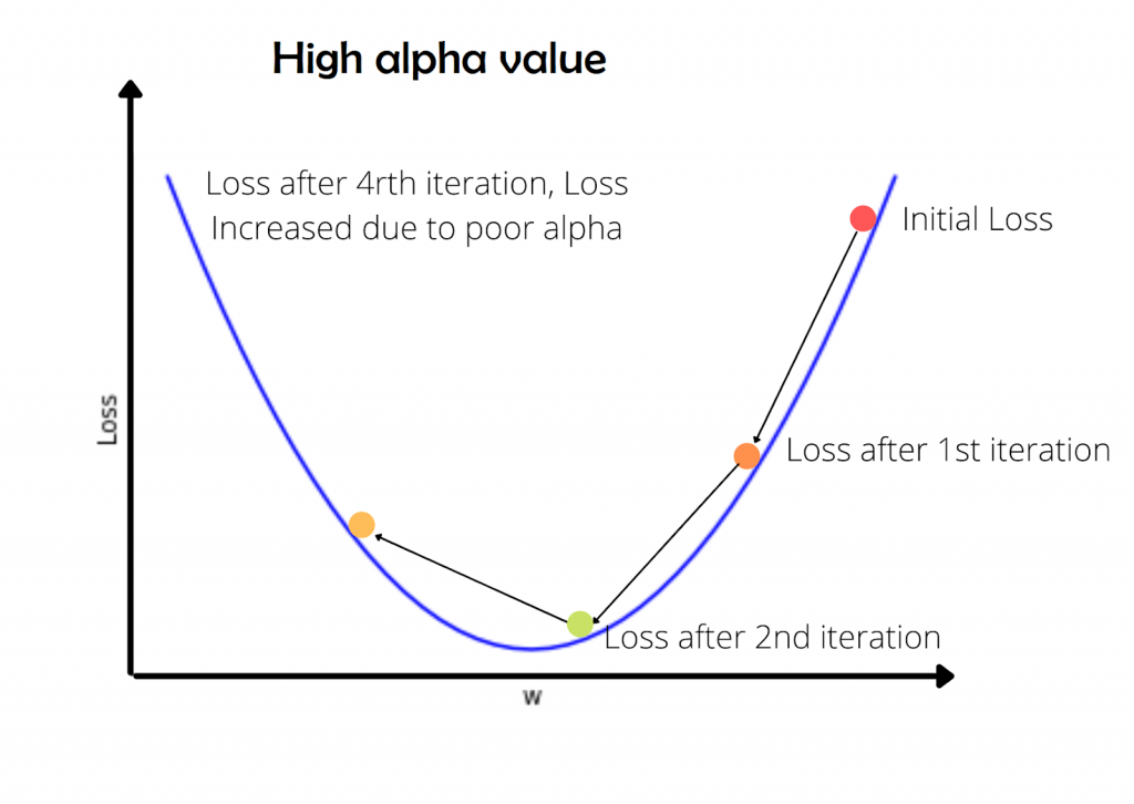
gradient descent with large learning rate

On the other hand, the high value of alpha will try to learn faster. But the loss will not converge as the step size (alpha) is large enough to escape the optimal loss. The high value of alpha refers to alpha values that are close to 0.1 to 1.

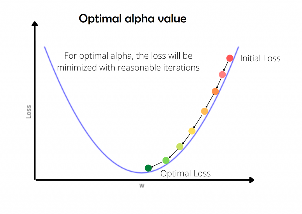
gradient descent with optimal learning rate

The optimal value of alpha is chosen highly based on the model you have, and the problem statement. This is an experimental value and needs to be found via experimentation.

Let’s understand this more intuitively by animations

We need to find W, b values so that the line W^TX+b can fit the data, that is W^TX+b ~= y. (here, ~= refers to approximately equal).

The below animations shows how the loss, W and b are changed (the slope and intercept of line)

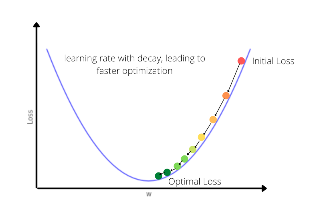
Now, instead of taking a single value of alpha can’t we update the alpha or learning rate with the iterations? That’s nothing but a decay value. Here as the loss minimizes, the value of the learning rate decreases. The formula will look like

Graphically we can see the process of this algorithm as

The equation for adaptive learning rate can be given by

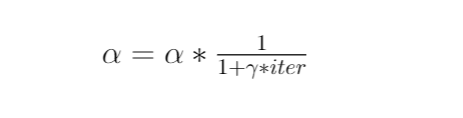
Where decay(gamma variable) is the parameter that ranges usually from 0 to 1. Higher the iteration lower will be the learning rate. This equation tries to decrease the learning rate as it goes near to optimal loss.

The python code for the same is as below:

    

import numpy as np
 
 
def gradient_descent(W, b, alpha, dW, db):
    '''
    Gradient Descent Algorithm:
    W : Weight term
    b : bias term
    alpha : learning rate
    dW : partial derivative of W value
    db : partial derivative of b value
    	    '''
    W = W - alpha * dW
    b = b - alpha * db
    return W,b
 
def cost(W, b, y, m):
    return 1/m * np.sum((np.dot(W.T,X.T)+b - y.T)**2)
 
X = np.array([i for i in range(5)]).reshape(-1,1)
 
arr1 = np.random.random(5)
y = (2*np.array([i for i in range(5)]) + arr1 * 1).reshape(-1,1)
 
print(X, y)
 
W = np.array([0]).reshape(-1,1)
b = np.array([0]).reshape(-1,1)
 
iterations = 7
alpha = 0.01
 
COST = []
# The transpose for X and W are done to adjust the dimension 
for i in range(iterations):
   
   dW = 1* np.dot(np.dot(W.T,X.T)+b - y.T, X)
   db = 1* np.sum(np.dot(W.T,X.T)+b - y.T)
   W, b = gradient_descent(W, b, alpha, dW, db)
   print(W, b)
   COST.append(cost(W, b, y, 5))

The above gradient descent algorithm is also known as Batch gradient descent since we are using all the data at once to learn the weights (entire batch).

For a smaller size of data, this will work smoothly, but when there is a humongous amount of data (In the range of millions), the computer may not be able to load such a large amount of data at once and the processing cannot be processed.

Ideally, if the number of data samples is less than 2000, then using batch gradient descent will be okay otherwise the problem may occur either in time or processing. To avoid these issues there are some widely used modifications to the algorithm as below.

Stochastic Gradient Descent
Mini-Batch Gradient Descent

Stochastic Gradient Descent

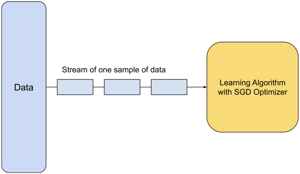
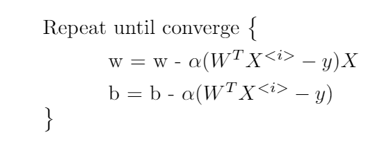
SGD is an abbreviation for stochastic gradient descent. SGD algorithm is also known as online learning since it learns by taking one sample of data at a time. We can understand it with the below diagram:

The algorithm can be equated as

One of the advantages of SGD is, SGD can be used for adaptive learning. For the data which are flowing continuously, the model needs to learn as quickly as possible. Situations like covid-19 case predictions need real-time data and the model needs to update quickly.

And here come some disadvantages, using SGD for offline learning (that is, we train the model after a bunch of data is collected) can be time-consuming. Also, the loss v/s iterations may not have a smooth curve since the data can vary a lot from sample to sample in each iteration.

The python code for this can be given as (only need to change in the iteration side):

    

import numpy as np
 
 
def gradient_descent(W, b, alpha, dW, db):
    '''
    Gradient Descent Algorithm:
    W : Weight term
    b : bias term
    alpha : learning rate
    dW : partial derivative of W value
    db : partial derivative of b value
    	    '''
    W = W - alpha * dW
    b = b - alpha * db
    return W,b
 
def cost(W, b, y, m):
    return 1/m * np.sum((np.dot(W.T,X.T)+b - y.T)**2)
 
X = np.array([i for i in range(5)]).reshape(-1,1)
 
arr1 = np.random.random(5)
y = (2*np.array([i for i in range(5)]) + arr1 * 1).reshape(-1,1)
 
print(X, y)
 
W = np.array([0]).reshape(-1,1)
b = np.array([0]).reshape(-1,1)
 
iterations = 7
alpha = 0.01
 
COST = []
# The transpose for X and W are done to adjust the dimension 
for i in range(iterations):
    dW = 1* np.dot(np.dot(W.T,X.T)+b - y.T, X)
    db = 1* np.sum(np.dot(W.T,X.T)+b - y.T)
    W, b = gradient_descent(W, b, alpha, dW, db)
    print(W, b)
    COST.append(cost(W, b, y, 1))

Mini-Batch Gradient Descent

Mini-Batch GD is the combination of SGD and Batch gradient descent. Instead of taking entire data or taking single sample data here, the data is in batches. The performance increases drastically for the deep learning models. Mini-batch is fast, and the data can be loaded quickly (as it has small samples of data). Usually, the batch sizes are in power of 2 but there are no hard rules.

The equation of this can be given as

The python code for mini-batch gradient descent

    

import numpy as np
 
 
def gradient_descent(W, b, alpha, dW, db):
    '''
    Gradient Descent Algorithm:
    W : Weight term
    b : bias term
    alpha : learning rate
    dW : partial derivative of W value
    db : partial derivative of b value
    	    '''
    W = W - alpha * dW
    b = b - alpha * db
    return W,b
 
def cost(W, b, y, m):
    return 1/m * np.sum((np.dot(W.T,X.T)+b - y.T)**2)
 
X = np.array([i for i in range(5)]).reshape(-1,1)
 
arr1 = np.random.random(5)
y = (2*np.array([i for i in range(5)]) + arr1 * 1).reshape(-1,1)
 
print(X, y)
 
W = np.array([0]).reshape(-1,1)
b = np.array([0]).reshape(-1,1)
 
iterations = 7
alpha = 0.01
 
COST = []
batch_size = 64 
for i in range(iterations):
    X = X[i*batch_size:(i+1)*batch_size]
    y = y[i*batch_size:(i+1)*batch_size]
    dW = 1* np.dot(np.dot(W.T,X.T)+b - y.T, X)
    db = 1* np.sum(np.dot(W.T,X.T)+b - y.T)
    W, b = gradient_descent(W, b, alpha, dW, db)
    print(W, b)
    COST.append(cost(W, b, y, batch_size))

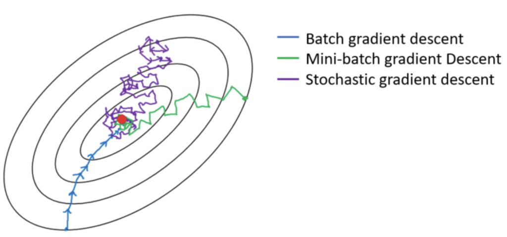
Gradient Descent Algorithms Comparison

To compare the Batch gradient descent, stochastic gradient descent, and mini-batch gradient descent algorithms, let’s make a contour plot of loss v/s iteration and a table.

Batch Gradient Descent	Stochastic Gradient Descent	Mini-Batch Gradient Descent
Time taken for each iteration is high	Time taken for each iteration is very low	Time taken for each iteration is higher than SGD but very less than Batch GD
Time taken to load the data is high (vectorization)	Time taken to load the data is low (vectorization)	Time taken to load the data is optimal (vectorization)
Iterations to reach the optimal loss is less (refer to above figure)	Iterations to reach the optimal loss is very high (refer to above figure)	Iterations to reach the optimal loss is reasonable (refer to above figure)
Suitable for data with samples below 2000	Suitable for online learning algorithms	Suitable for data with huge size, which need not be online

So, till now we have gone through basic variants of gradient descent. It’s time to explore some advanced optimization algorithms that are used widely in deep learning. We are going to cover these 3 in this article.

Momentum optimization
RMS prop optimization
Adam optimization

Why do we need other optimization algorithms when we have something like mini-batch gradient descent? The reason is the training speed (number of iterations to converge).

In most cases, if trained with direct Mini Batch gradient descent, the training will be slow. (For a humongous amount of data). Researchers have developed few algorithm variants to speed up the training process of deep learning models.

Loss functions for Classification Algorithms

Relevant Article

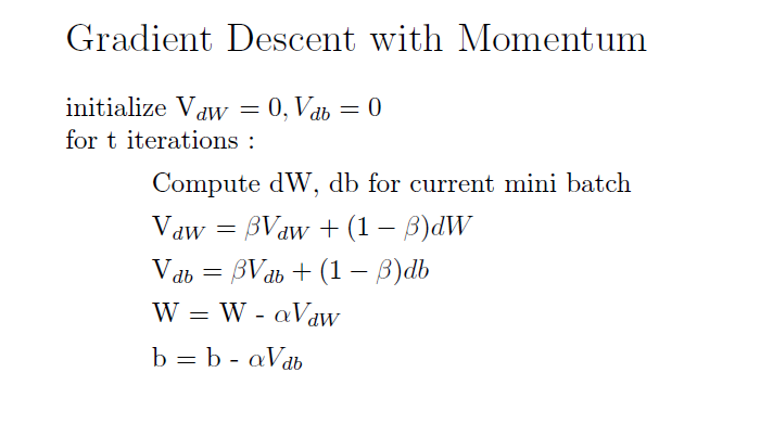
Guide to Classification Loss Function for Machine Learning

Gradient Descent with Momentum

As the words say, it provides the gradient descent a momentum to converge faster. The Algorithm can be given as.

Let’s understand this in-depth

Firstly initializing the weights and Vdw, Vdb terms. Here Vdw and Vdb are the variables that are responsible for the actual momentum. Here β is the hyperparameter which needs to be chosen for better optimization. From the Vdw and Vdb, we are computing the updated W and b with the learning rate.

Why does it work?

It works because equations 1 and 2 will carry the information from the previous iteration. In the updation step, the new Vdw/Vdb is the sum of β times Vdw/Vdb and (1- Vdw/Vdb) times the changed value of weights/bias.

Because it utilises the value from previous step, the learning is more adoptive and thus fast compared a normal mini-batch algorithm. Generally β is set to 0.9, it works in most cases.

The pseudo python Code for this can be given as below.

    
import numpy as np
def momentum(X, y, batch_size, W, b, alpha, beta, dW, db, iterations):
    VdW = 0
    Vdb = 0
    
    for i in range(iterations):
        X = X[i*batch_size:(i+1)*batch_size]
        y = y[i*batch_size:(i+1)*batch_size]
 
        dW = derivative(W) #Based on the loss function
        db = derivative(b) #Based on the loss function
 
        VdW = beta*VdW + (1-beta) * dW
        Vdb = beta*Vdb + (1-beta) * db
 
        W = W - alpha * (1/batch_size) * VdW
        b = b - alpha * (1/batch_size) * Vdb
           
    return W, b

RMS Prop

RMS Prop stands for Root Mean Square Propagation. Similar to momentum, the RMSprop provides a boost to the gradient descent to converge faster. The algorithm can be written as below:

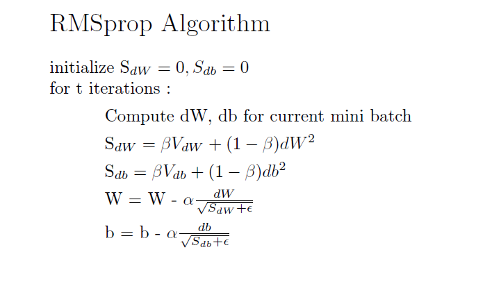
Note: In the equation, Vdw and Vdb should be Sdw and Sdb after equal sign

Here Sdw and Sdb are the intermediate modifiers that speed up the conversion. The term dW2_square is the differentiation of loss. Here β plays the similar role, to get the weighted average of the past values.

β is generally kept as 0.99 for RMS prop. Next, the W and b are updated with learning rate. (refer the diagram)

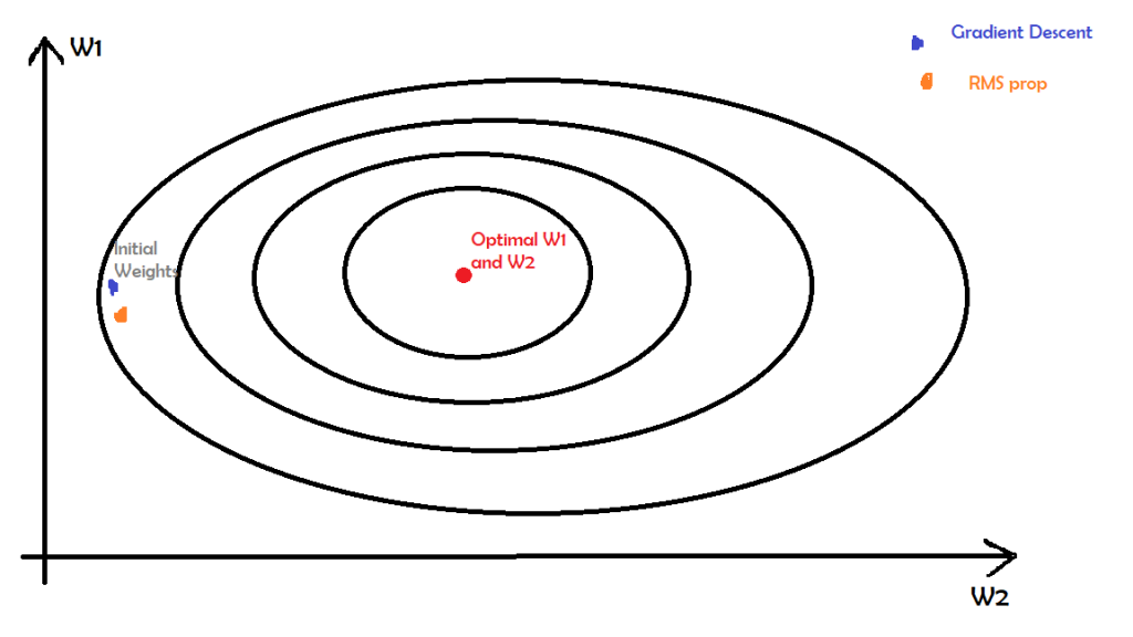
The RMS prop will increase the learning for weights/bias that are away from the optimal value. Here W1 and W2 seems away from the optimal value. So, the RMS prop will increase the value of S to move the weight near to optimal weights. The below figure shows the same.

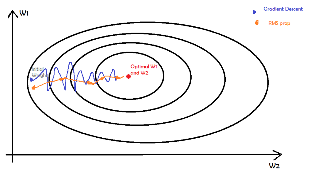
The gradient descent will oscillate a lot to find the optimal W1, W2. But, the RMSprop will converge to the optimal W1, W2 comparatively sooner using the past values.

Also, to avoid division by zero or the division by a really small number, we add epsilon- a very small value (in order of 10^-8) to the Sdw and Sdb.

The pseudo python Code for the same:

    
import numpy as np
def RMSprop(X, y, batch_size, W, b, alpha, beta, dW, db, epochs, epsilon= 1e-8):
    SdW = 0
    Sdb = 0
    for i in range(epochs):
 
        X = X[i*batch_size:(i+1)*batch_size]
        y = y[i*batch_size:(i+1)*batch_size]
 
        dW = derivative(W) #Based on the loss function
        db = derivative(b) #Based on the loss function
 
        SdW = beta*SdW + (1-beta) * dW**2
        Sdb = beta*Sdb + (1-beta) * db**2
 
        W = W - alpha * (1/batch_size) * dW/(np.sqrt(SdW) + epsilon)
        b = b - alpha * (1/batch_size) * db/(np.sqrt(Sdb) + epsilon)
           
    return W, b

Adam Optimizer

Adam Optimization is the combination of both Momentum and RMS prop algorithms. Adam stands for ADAptive Moment Optimization.

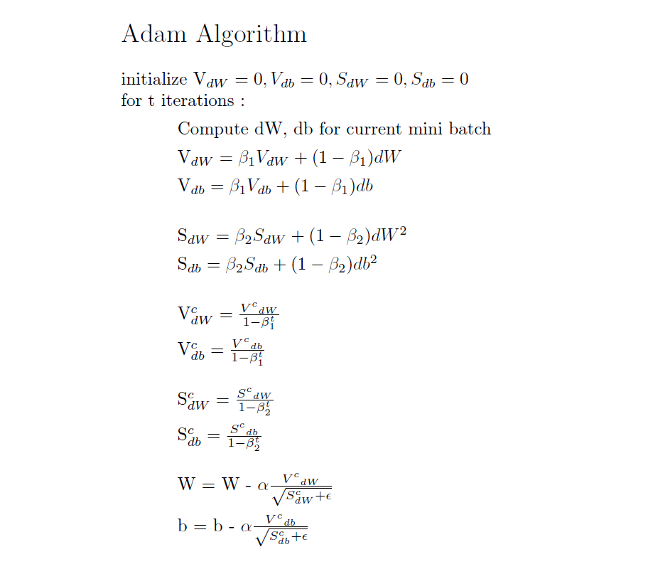
The term Vdw corresponds to the momentum, and Sdw corresponds to the RMSprop. Let’s understand step wise.

Compute Vdw and Vdb values from their past values (similar to momentum). Here β1 is a hyper parameter for the equation.
Compute Sdw and Sdb values from their past values (similar to RMSprop). Here 2 is the weight of the equation.
Next, Vdw, Vdb, Sdw, and Sdb values are corrected using dw, db, β1, and β2. This is done for bias correction.
Finally, the W, b values are computed using the final equation.

Here is the detail about hyperparameters.

α(alpha) : This parameter is the learning rate, similar to other gradient descent variants. Generally, we need to tune the parameter based on the model and problem statements.

β1 (beta 1) : This parameter is due to the momentum equation that involves the dW, db terms. Generally, the beta 1 is set to 0.9

β2 (beta 2) : This parameter is due to the RMS prop equation that involves the dW2, db2 terms. Generally, the beta 2 is set to 0.999

ε(epsilon) : This parameter is to avoid the blowing up of the final equation. If Sdw corrected is too small, the term will tend to reach infinity( very high value). Generally, epsilon is set to 10-8.

The pseudo python Code for this

    
import numpy as np
def Adam(X, y, batch_size, W, b, alpha, dW, db, epochs, beta1=0.9, beta2=0.999, epsilon= 1e-8):
    SdW = 0
    Sdb = 0
    for i in range(epochs):
 
        X = X[i*batch_size:(i+1)*batch_size]
        y = y[i*batch_size:(i+1)*batch_size]
 
        dW = derivative(W) #Based on the loss function
        db = derivative(b) #Based on the loss function
 
        VdW = beta2*VdW + dW
        Vdb = beta2*Vdb + db
 
        SdW = beta1*SdW + dW**2
        Sdb = beta1*Sdb + db**2
 
        VdW_corrected = VdW/(1-beta1**(i+1)) #instead of i use i+1 to resolve i=0 issue
        Vdb_corrected = Vdb/(1-beta1**(i+1)) #instead of i use i+1 to resolve i=0 issue
 
        SdW_corrected = SdW/(1-beta2**(i+1))
        Sdb_corrected = Sdb/(1-beta2**(i+1))
 
        W = W - alpha * (1/batch_size) * VdW_corrected/(np.sqrt(SdW_corrected) + epsilon)
        b = b - alpha * (1/batch_size) * Vdb_corrected/(np.sqrt(Sdb_corrected) + epsilon)
           
    return W, b

Adam is one the powerful optimization algorithms, which is used widely by both in industry and academia. Also, adam optimization is widely used across multiple problem statements since it generalises well.

Awesome! We have come to the conclusion now. To the quick summarise, we have understood the basics of gradient descent. What are its basic variants including Stochastic gradient descent, Mini Batch gradient descent. Also, we have learnt some of the advanced algorithms like Momentum, RMSprop and Adam optimizer.

Navaneeth Sharma

Navaneeth Sharma is a content contributor at DataMonje. He is passionate about Artificial intelligence. Navaneeth has contributed to publishing two machine learning integrated pip packages Scrapegoat and AksharaJaana. He aims to become a full-time AI Research Engineer.

Cookie	Duration	Description
cookielawinfo-checkbox-analytics	11 months	This cookie is set by GDPR Cookie Consent plugin. The cookie is used to store the user consent for the cookies in the category "Analytics".
cookielawinfo-checkbox-functional	11 months	The cookie is set by GDPR cookie consent to record the user consent for the cookies in the category "Functional".
cookielawinfo-checkbox-necessary	11 months	This cookie is set by GDPR Cookie Consent plugin. The cookies is used to store the user consent for the cookies in the category "Necessary".
cookielawinfo-checkbox-others	11 months	This cookie is set by GDPR Cookie Consent plugin. The cookie is used to store the user consent for the cookies in the category "Other.
cookielawinfo-checkbox-performance	11 months	This cookie is set by GDPR Cookie Consent plugin. The cookie is used to store the user consent for the cookies in the category "Performance".
viewed_cookie_policy	11 months	The cookie is set by the GDPR Cookie Consent plugin and is used to store whether or not user has consented to the use of cookies. It does not store any personal data.